BDNYC Database Setup

WARNING: The information on this is outdated. We recommend looking into the up-to-date documentation at trac (internal) and ReadTheDocs.

Read this post first if your development environment needs setting up. Then…

Setting Up the Database

To install the database, open a Terminal session and do:

pip install BDNYCdb

Then download the public database file BDNCY198.db here or get the unpublished BDNYC.db file from Dropbox. (Ask a group member for the invite!)

Accessing the Database

Now you can load the entire database into a Python variable simply by launching the Python interpreter and pointing the get_db() function to the database file by doing:

In [1]: from BDNYCdb import BDdb
In [2]: db = BDdb.get_db('/path/to/your/Dropbox/BDNYCdb/BDNYC.db')

Voila!

In the database, each source has a unique identifier (or ‘primary key’ in SQL speak). To see an inventory of all data for one of these sources, just do:

In [3]: db.inventory(id)

where id is the source_id.

Now that you have the database at your fingertips, you’ll want to get some info out of it. To do this, you can use SQL queries.

Here is a detailed post about how to write an SQL query.

Further documentation for sqlite3 can be found here. Most commands involve wrapping SQL language inside python functions. The main method we will use to fetch data from the database is list():

In [5]: data = db.list( "SQL_query_goes_here" ).fetchall()

Example Queries

Some SQL query examples to put in the command above (wrapped in quotes of course):

  1. SELECT shortname, ra, dec FROM sources WHERE (222<ra AND ra<232) AND (5<dec AND dec<15)
  2. SELECT band, magnitude, magnitude_unc FROM photometry WHERE source_id=58
  3. SELECT source_id, band, magnitude FROM photometry WHERE band=’z’ AND magnitude<15
  4. SELECT wavelength, flux, unc FROM spectra WHERE observation_id=75”

As you hopefully gathered:

  1. Returns the shortname, ra and dec of all objects in a 10 square degree patch of sky centered at RA = 227, DEC = 10
  2. Returns all the photometry and uncertainties available for object 58
  3. Returns all objects and z magnitudes with z less than 15
  4. Returns the wavelength, flux and uncertainty arrays for all spectra of object 75

The above examples are for querying individual tables only. We can query from multiple tables at the same time with the JOIN command like so:

  1. SELECT t.name, p.band, p.magnitude, p.magnitude_unc FROM telescopes as t JOIN photometry AS p ON p.telescope_id=t.id WHERE p.source_id=58
  2. SELECT p1.magnitude-p2.magnitude FROM photometry AS p1 JOIN photometry AS p2 ON p1.source_id=p2.source_id WHERE p1.band=’J’ AND p2.band=’H’
  3. SELECT src.designation, src.unum, spt.spectral_type FROM sources AS src JOIN spectral_types AS spt ON spt.source_id=src.id WHERE spt.spectral_type>=10 AND spt.spectral_type<20 AND spt.regime=’optical’
  4. SELECT s.unum, p.parallax, p.parallax_unc, p.publication_id FROM sources as s JOIN parallaxes AS p ON p.source_id=s.id

As you may have gathered:

  1. Returns the survey, band and magnitude for all photometry of source 58
  2. Returns the J-H color for every object
  3. Returns the designation, U-number and optical spectral type for all L dwarfs
  4. Returns the parallax measurements and publications for all sources

Alternative Output

As shown above, the result of a SQL query is typically a list of tuples where we can use the indices to print the values. For example, this source’s g-band magnitude:

In [9]: data = db.list("SELECT band,magnitude FROM photometry WHERE source_id=58").fetchall()
In [10]: data
Out[10]: [('u', 25.70623),('g', 25.54734),('r', 23.514),('i', 21.20863),('z', 18.0104)]
In [11]: data[1][1]
Out[11]: 25.54734

However we can also query the database a little bit differently so that the fields and records are returned as a dictionary. Instead of db.query.execute() we can do db.dict() like this:

In [12]: data = db.dict("SELECT * FROM photometry WHERE source_id=58").fetchall()
In [13]: data
Out[13]: [<sqlite3.Row at 0x107798450>, <sqlite3.Row at 0x107798410>, <sqlite3.Row at 0x107798430>, <sqlite3.Row at 0x1077983d0>, <sqlite3.Row at 0x1077982f0>]
In [14]: data[1]['magnitude']
Out[14]: 25.54734

Database Schema and Browsing

In order to write the SQL queries above you of course need to know what the names of the tables and fields in the database are. One way to do this is:

In [15]: db.list("SELECT sql FROM sqlite_master").fetchall()

This will print a list of each table, the possible fields, and the data type (e.g. TEXT, INTEGER, ARRAY) for that field.

SQL browser
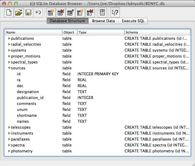
Even easier is to use the DB Browser for SQLite pictured at left which lets you expand and collapse each table, sort and order columns, and other fun stuff.

It even allows you to manually create/edit/destroy records with a very nice GUI.

IMPORTANT: If you are using the private database keep in mind that if you change a database record, you immediately change it for everyone since we share the same database file on Dropbox. Be careful!

Always check and double-check that you are entering the correct data for the correct source before you save any changes with the SQLite Database Browser.

SQL Queries

An SQL database is comprised of a bunch of tables (kind of like a spreadsheet) that have fields (column names) and records (rows of data). For example, our database might have a table called students that looks like this:

id first last grade GPA
1 Al Einstein 6 2.7
2 Annie Cannon 6 3.8
3 Artie Eddington 8 3.2
4 Carlie Herschel 8 3.2

So in our students table, the fields are [id, first, last, grade, GPA], and there are a total of four records, each with a required yet arbitrary id in the first column.

To pull these records out, we tell SQL to SELECT values for the following fields FROM a certain table. In SQL this looks like:

In [1]: db.execute("SELECT id, first, last, grade, GPA FROM students").fetchall()
Out[1]: [(1,'Al','Einstein',6,2.7),(2,'Annie','Cannon',6,3.8),(3,'Artie','Eddington',8,3.2),(4,'Carlie','Herschel',8,3.2)]

Or equivalently, we can just use a wildcard “*” if we want to return all fields with the SQL query "SELECT * FROM students".

We can modify our SQL query to change the order of fields or only return certain ones as well. For example:

In [2]: db.execute("SELECT last, first, GPA FROM students").fetchall()
Out[1]: [('Einstein','Al',2.7),('Cannon','Annie',3.8),('Eddington','Artie',3.2),('Herschel','Carlie',3.2)]

Now that we know how to get records from tables, we can restrict which records it returns with the WHERE statement:

In [3]: db.execute("SELECT last, first, GPA FROM students WHERE GPA>3.1").fetchall()
Out[3]: [('Cannon','Annie',3.8),('Eddington','Artie',3.2),('Herschel','Carlie',3.2)]

Notice the first student had a GPA less than 3.1 so he was omitted from the result.

Now let’s say we have a second table called quizzes which is a table of every quiz grade for all students that looks like this:

id student_id quiz_number score
1 1 3 89
2 2 3 96
3 3 3 94
4 4 3 92
5 1 4 78
6 3 4 88
7 4 4 91

Now if we want to see only Al’s grades, we have to JOIN the tables ON some condition. In this case, we want to tell SQL that the student_id (not the id) in the quizzes table should match the id in the students table (since only those grades are Al’s). This looks like:

In [4]: db.execute("SELECT quizzes.quiz_number, quizzes.score FROM quizzes JOIN students ON students.id=quizzes.student_id WHERE students.last='Einstein'").fetchall()
Out[4]: [(3,89),(4,78)]

So students.id=quizzes.student_id associates each quiz with a student from the students table and students.last='Einstein' specifies that we only want the grades from the student with last name Einstein.

Similarly, we can see who scored 90 or greater on which quiz with:

In [5]: db.execute("SELECT students.last, quizzes.quiz_number, quizzes.score FROM quizzes JOIN students ON students.id=quizzes.student_id WHERE quizzes.score>=90").fetchall()
Out[5]: [('Cannon',3,96),('Eddington',3,94),('Herschel',3,92),('Herschel',4,91)]

That’s it! We can JOIN as many tables as we want with as many restrictions we need to pull out data in the desired form.

This is powerful, but the queries can become lengthy. A slight shortcut is to use the AS statement to assign a table to a variable (e.g. students => s, quizzes => q) like such:

In [6]: db.execute("SELECT s.last, q.quiz_number, q.score FROM quizzes AS q JOIN students AS s ON s.id=q.student_id WHERE q.score>=90").fetchall()
Out[6]: [('Cannon',3,96),('Eddington',3,94),('Herschel',3,92),('Herschel',4,91)]

Ground Based Photometry

Here I want to calculate some photometric points from spectra for comparison with published values for a bunch of known brown dwarfs.

In order to get the true magnitude $$m$$ for an object, I first need to calculate the instrumental magnitude $$m_\text{inst}$$ and then correct for a number of effects. That is, I calculate the apparent magnitude from a particular place on the Earth and then add corrections to determine what it would be if we measured from space.

After all our corrections are made, the magnitude is given by:

$$!m=m_\text{inst}-ZP_m-k_m\cdot X$$

Instrumental Magnitude

The first term on the right in the equation above is the magnitude measured by the instrument on the ground, given by:

$$!m_\text{inst}=-2.5\log\left(\int f_\lambda (\lambda)\left(\frac{\lambda}{hc}\right)S_m(\lambda)d\lambda\right)$$

Where $$f_\lambda (\lambda)$$ is the energy flux density of the source in units of [erg s-1 cm-2 A-1] and $$S_m(\lambda)$$ is the scalar filter throughput for the band of interest.

Since I will be comparing my calculated magnitudes to photometry taken with photon counting devices, the factor of $$\frac{\lambda}{hc}$$ converts $$f_\lambda (\lambda)$$ to a photon flux density in units [photons s-1 cm-2 A-1].

Zero Point Correction

The second term in our magnitude equation is a first order correction to compare $$m_\text{inst}$$ to some standard we define as zero. I will use a flux calibrated spectrum of the A0 star Vega to calculate the zero point magnitude for the band:

$$!ZP_m=-2.5\log\left(\int f_{\lambda\text{ Vega}}(\lambda)\left(\frac{\lambda}{hc}\right)S_m(\lambda)d\lambda\right)$$

Just as we obtained our instrumental magnitude above.

Extinction Correction

The third term is to correct for the extinction of the source flux due to atmospheric absorption. We can get closer to the true apparent magnitude (above the atmosphere) by adding an extinction term:

$$!k_m\cdot\sec (z)=k_m\cdot X$$

Where $$k_m$$ is the extinction coefficient for the band of interest and $$\sec(z)=X$$ is the airmass.

The airmass is the optical path length of the atmosphere, which attenuates the source flux depending on its angle from the zenith $$z$$. Approximating the truly spherical atmosphere as plane-parallel, the airmass goes from $$X=1$$ at $$z=0^\circ$$ to $$X=2$$ at $$z=60^\circ$$. At zenith angles greater than that, the plane-parallel approximation falls apart and the airmass term gets complicated.

Where the airmass is the amount of atmosphere in the line of sight, the extinction coefficient is the amount by which the incident light is attenuated as it travels through the airmass. The extinction coefficient is related to the optical depth $$\tau$$ of the atmosphere as:

$$!m-m_0=-2.5\log\left(\frac{I}{I_0}\right)=-2.5\log (e^{-\tau X})=1.086\cdot\tau\cdot X=k_m\cdot X$$

Where $$m$$ and $$m_0$$ are the magnitudes below and above the atmosphere respectively.

Example: J21512543-2441000

As an example, I’d like to calculate the 2MASS J-band magnitude of the brown dwarf at 21h51m25.43s -24d41m00s given a low resolution NIR energy flux density from the SpeX Prism instrument on the 3m NASA Infrared Telescope Facility.

J21512543-2441000

Interpolating the filter throughput to the object spectrum and then integrating as in the equation above, I get $$J_\text{inst}=10.046$$ as my instrumental magnitude in the J-band.

Performing the same procedure on the flux calibrated spectrum of Vega, I get $$ZP_J=-5.721$$ for my J-band zero point magnitude.

Checking the FITS file header, I will use $$X=1.444625$$ for the airmass. The mean extinction coefficient for the MKO system J-band is given as $$k_J=0.0153$$ in Tokunaga & Vacca (2007), making the atmospheric correction term $$k_J\cdot X=0.0221$$.

The corrected magnitude is then:

$$!J=J_\text{inst}-ZP_J-k_J\cdot X=10.046-(-5.721)-0.0221=15.745$$

Which is only 0.007 magnitudes off from the value of $$J=15.752$$ from the 2MASS catalog.

Remaining Problems

As shown in the example above, this works… but not for every object.

2MASS apparent J magnitudes vs. my calculated apparent j magnitudes for 67 brown dwarfs. The solid black line is for perfect agreement and the dashed line is a best fit of the data.

2MASS apparent J magnitudes vs. my calculated apparent j magnitudes for 67 brown dwarfs. The solid black line is for perfect agreement and the dashed line is a best fit of the data.

2MASS apparent H magnitudes vs. my calculated apparent h magnitudes for 67 brown dwarfs. The solid black line is for perfect agreement and the dashed line is a best fit of the data.

2MASS apparent H magnitudes vs. my calculated apparent h magnitudes for 67 brown dwarfs. The solid black line is for perfect agreement and the dashed line is a best fit of the data.

I whittled down my sample of 875 to only those objects with flux units and airmass values taken at Mauna Kea so that I could use the same extinction coefficient and make sure they are all in the same units of [erg s-1 cm-2 A-1].

Then I pulled the 2MASS catalog J and H magnitudes with uncertainties for these remaining objects and plotted them against my calculated values with uncertainties.

To the left are the plots of the 67 objects that fit the selection criteria in J-band (above) and H-band (below).

Though it’s not the biggest sample, the deviation of the best fit line from unity suggests I’m off by a factor of 0.9 from the 2MASS catalog value across the board.

But more worrisome is the fact that most of the calculated magnitudes are not within the errors of the 2MASS magnitudes. This deviation ranges from very good agreement of a few thousandths of a magnitude up to the worst offenders of about 0.8 mags.

Filter Effective Wavelength(s)

The effective wavelength of a filter for narrow band photometry can easily be approximated by a constant and just looked up when needed. For broad band photometry, however, the width of the filter and the amount of flux in the band being measured actually come into play.

The effective wavelength of a filter is given by:

$$!\lambda_\text{eff}=\frac{\int \lambda \text{ }f_\lambda (\lambda)\text{ }S(\lambda)\text{ } d\lambda}{\int f_\lambda (\lambda)\text{ } S(\lambda)\text{ } d\lambda}$$

Where $$S(\lambda)$$ is the scalar filter throughput and $$f_\lambda$$ is the flux density in units of [erg s-1 cm-2 A-1] or [photons s-1 cm-2 A-1] depending upon whether you are using an energy measuring or a photon counting detector, respectively.

Here are the results for 67 brown dwarfs with complete spectrum coverage of the 2MASS J-band:

Effective wavelength values for the 2MASS J-band filter. Blue and green circles indicate lambda calculated using photon flux densities (PFD) and energy flux densities (EFD) respectively. Filled circles are for 67 confirmed brown dwarfs. Open circles are for Vega.

Effective wavelength values for the 2MASS J-band filter. Blue and green circles indicate lambda calculated using photon flux densities (PFD) and energy flux densities (EFD) respectively. Filled circles are for 67 confirmed brown dwarfs. Open circles are for Vega.

The red line on the plot shows the specified value given by 2MASS. For fainter objects like brown dwarfs (filled circles), the calculated effective wavelength of the J-band filter can shift redward by as much as 150 angstroms. Vega (open circles) shifts it blueward by about 30 angstroms.

The difference is small but measurable and demonstrates the dependence of the filter width, source spectrum, and detector type on the effective wavelength $$\lambda_\text{eff}$$ while doing broad band photometry.

Visualizing results from low-res NIR spectral fits

In my first serious foray into Python and github I adapted some plotting code from Dan Foreman_Mackey with the help of Adrian Price-Whelan  and Joe Filippazzo to create contour plots and histograms of my fitting results! These are histograms MCMC results for model fits to a low-resolution near-infrared spectrum of a young L5 brown dwarf, in temperature and gravity atmospheric parameters. The colors represent different segments of the spectrum – purple is YJH, blue is YJ, red is H. The take-away is that different segments of the spectrum results in different temperatures, and all parts of the spectrum make it look old (high gravity). This is probably because the overly-simplistic dust treatments in the models are not sufficient for young, low-mass objects.

L5_young_JH_J_H_rotate

The baseline for comparison is the result for a field L5 dwarf, shown below. The temperatures are much more consistent with one another and what you would expect for an L5 spectral type from other methods, and the gravities are similarly high (although too high for comfort for J band). This is reassuring for the method in general and probably means that we need most sophisticated dust treatments in the models to handle giant-exoplanet-like young brown dwarfs. Paper will be submitted soon!

L5_JH_J_H_rotate

Photon Flux Density vs. Energy Flux Density

One of the subtleties of photometry is the difference between magnitudes and colors calculated using energy flux densities (EFD) and photon flux densities (PFD).

The complication arises since the photometry presented by many surveys is calculated using PFD but spectra (specifically the synthetic variety) is given as EFD. The difference is small but measurable so let’s do it right.

The following is the process I used to remedy the situation by switching my models to PFD so they could be directly compared to the photometry from the surveys. Thanks to Mike Cushing for the guidance.

Filter Zero Points

Before we can calculate the magnitudes, we need filter zero points calculated from PFD. To do this, I started with a spectrum of Vega in units of [erg s-1 cm-2 A-1] snatched from STSci.

Then the zero point flux density in [photons s-1 cm-2 A-1] is:

$$!F_{zp}=\frac{\int p_V(\lambda) S(\lambda) d\lambda}{\int S(\lambda)d\lambda}=\frac{\int e_V(\lambda)\left( \frac{\lambda}{hc}\right) S(\lambda) d\lambda}{\int S(\lambda)d\lambda}$$

Where $$e_V$$ is the given energy flux density in [erg s-1 cm-2 A-1] of Vega, $$p_V$$ is the photon flux density in [photons s-1 cm-2 A-1], and $$S(\lambda)$$ is the scalar filter throughput.

Since I’m starting with a spectrum of Vega in EFD units, I need to multiply by $$\frac{\lambda}{hc}$$ to convert it to PFD units.

In Python, this looks like:

def zp_flux(band):
    from scipy import trapz, interp, log10
    (wave, flux), filt, h, c = vega(), get_filters()[band], 6.6260755E-27 # [erg*s], 2.998E14 # [um/s]
    I = interp(wave, filt['wav'], filt['rsr'], left=0, right=0)
    return trapz(I*flux*wave/(h*c), x=wave)/trapz(I, x=wave))

Calculating Magnitudes

Now that we have the filter zero points, we can calculate the magnitudes using:

$$!m = -2.5\log\left(\frac{F_\lambda}{F_{zp}}\right)$$

Where $$m$$ is the apparent magnitude and $$F_\lambda$$ is the flux from our source given similarly by:

$$!F_{\lambda}=\frac{\int p_\lambda(\lambda) S(\lambda) d\lambda}{\int S(\lambda)d\lambda}=\frac{\int e_\lambda(\lambda)\left( \frac{\lambda}{hc}\right) S(\lambda) d\lambda}{\int S(\lambda)d\lambda}$$

Since the synthetic spectra I’m using are given in EFD units, I need to multiply by $$\frac{\lambda}{hc}$$ to convert it to PFD units just as I did with my spectrum of Vega.

In Python the magnitudes are obtained the same way as above but we use the source spectrum in [erg s-1 cm-2 A-1] instead of Vega. Then the magnitude is just:

mag = -2.5*log10(source_flux(band)/zp_flux(band))

Below is an image that shows the discrepancy between using EFD and PFD to calculate colors for comparison with survey photometry.

The circles are colors calculated from synthetic spectra of low surface gravity (large circles) to high surface gravity (small circles). The grey lines are iso-temperature contours. The jumping shows the different results using PFD and EFD. The stationary blue stars, green squares and red triangles are catalog photometric points calculated from PFD.

The circles are colors calculated from synthetic spectra of low surface gravity (large circles) to high surface gravity (small circles). The grey lines are iso-temperature contours. The jumping shows the different results using PFD and EFD. The stationary blue stars, green squares and red triangles are catalog photometric points calculated from PFD.

Other Considerations

The discrepancy I get between the same color calculated from PFD and EFD though is as much as 0.244 mags (in r-W3 at 1050K), which seems excessive. The magnitude calculation reduces to:

$$!m = -2.5\log\left( \frac{\int e_\lambda(\lambda)S(\lambda) \lambda d\lambda}{\int e_V(\lambda) S(\lambda) \lambda d\lambda}\right)$$

Since the filter profile is interpolated with the spectrum before integration, I thought the discrepancy must be due only to the difference in resolution between the synthetic and Vega spectra. In other words, I have to make sure the wavelength arrays for Vega and the source are identical so the trapezoidal sums have the same width bins.

This reduces the discrepancy in r-W3 at 1050K from -0.244 mags to -0.067 mags, which is better. However, the discrepancy in H-[3.6] goes from 0.071 mags to -0.078 mags.

To Recapitulate

In summary, I had a spectrum of Vega and some synthetic spectra all in energy flux density units of [erg s-1 cm-2 A-1] and some photometric points from the survey catalogs calculated from photon flux density units of [photons s-1 cm-2 A-1].

In order to compare apples to apples, I first converted my spectra to PFD by multiplying by $$\frac{\lambda}{hc}$$ at each wavelength point before integrating to calculate my zero points and magnitudes.

Colors Diagnostic of Surface Gravity

The goal here is to find a prescription of colors diagnostic of brown dwarf surface gravity. Since early optical as well as far infrared spectra and photometry are uncommon, the bands of interest should only include i and z from SDSS; J, H and Ks from 2MASS; and W1, W2 and W3 (but not W4 with only 10 percent detection) from WISE.

In order to find said prescriptions, I used the BT-Settl models (at solar metallicity ranging from 1000 – 3000 K in effective temperature and 3.0 – 5.5 dex in log surface gravity) to produce a suite of color-color and color-parameter plots.

One method I employed was to choose one effective temperature (in this case 2500K) and anchor the colors in one band that doesn’t vary much between high and low surface gravity, e.g. z-band. Then I chose the other two bands by one that was more luminous at low gravity and one that was more luminous at high gravity, e.g. W2- and J-band respectively.

BT-Settl model spectra at 2500K

Then the color-color plot of these bands looks like:

In this plot of z-J vs. z-W2 the smallest circles are objects with high surface gravity and the largest have low surface gravity (log(g) = 5.5 to 3.5 respectively). The light grey lines are iso-temperature contours.

In this plot of z-J vs. z-W2 the smallest circles are objects with high surface gravity and the largest have low surface gravity (log(g) = 5.5 to 3.5 respectively). The light grey lines are iso-temperature contours.

In this particular case, there is little-to-no dispersion in z-J for Teff = 2500K (d = 0.009) and an appreciable dispersion in z-W2 for that same Teff (d = 0.32). Notice the tight vertical grouping (z-J) and dispersed horizontal grouping (z-W2) for the model objects of Teff = 2500K and varying log(g) in the red rectangle on the color-color plot above.

Double-checking with the color-Teff plots, we can see that the dispersion in z-J in the plot on the left is tiny and the horizontal offset in the color-color plot is due to the 0.32 magnitude dispersion in z-W2 on the right below.

Of course this is just a different way of looking at the same thing, but I might be able to find colors that are reliable indicators of gravity (and thus age) if I can find a bunch of these examples where the flux in the secondary and tertiary bands are flipped.

Of note is the fact that at this temperature in this color-color plot the points are also isolated, i.e. there are no degeneracies with objects of any other temperature. That means that if I find an object with a z-J = 1.65 or so, I know that it has an effective temperature of about 2500K. Then I can determine its age by seeing if its z-W2 color is closer to 3.3 (young) or 2.9 (old).

This of course does not work for all temperatures, as shown in the red circle in the color-color plot above. This demonstrates a degeneracy among hotter young objects (Teff = 3000K, log(g) = 3.5) and cooler old objects (Teff = 2800K, log(g) = 5.5) with a temperature difference of 200K.

Though there is no definitive combination of colors to identify the age of an object irrespective of temperature, what I have done here is found a collection of prescriptions that are reliable indicators of age over small temperature ranges.

Memory Leaks in Python

I just spent a few hours tracking down a massive memory leak in the Python code I’m working on for my current project.  Running the code on even a single object would eat up 4 GB of memory in my computer, and that slowed the entire system down to the point that other programs were unusable, even if they didn’t crash outright.  After fixing the memory leak, the memory usage stayed between 200-204 MB for the entire time the program was running.

As it turns out, the problem was that every loop was creating several plots, and (even though I was writing them to files) not closing them with a plt.clf() except after the end of the loop, which only affected the last plot object.

The gist of it is, there are only a few reasons for memory leaks in Python.

  1. There’s some object you are opening (repeatedly) but not closing.
  2. You are repeatedly adding data to a list/dict and not removing the old data. (for instance, if you’re appending data to an array instead of replacing the array)
  3. There’s a memory leak in one of the libraries you’re calling. (unlikely)

source: http://www.lshift.net/blog/2008/11/14/tracing-python-memory-leaks

I haven’t successfully tried the methods listed in the above link (they seem to be for heavier-duty programming than we use) but that first reason is likely to be a problem for BDNYC:  We open plot figures, we open the BDNYC database, we open .fits files with astropy… remember to close things properly.

For the record, this seems to be the correct sequence for making a matplotlib plot:

fig = pyplot.figure(1)
ax = fig.add_subplot(111) # or fig.add_axes()
ax.plot(<blah>)
ax.set_xlabel(<label>)
(...)
fig.savefig(<filename>)
fig.clf()
pyplot.close()

That last line was completely new to me, but is apparently necessary if you do it this way.  Matplotlib works without creating a figure, adding axes to a figure, and then adding plot commands to the axis… but if used this way, you can actually edit multiple figures and their subplots at the same time — just specify which axis variable you want to add the plot element to. To my knowledge, this is a clear advantage over IDL: IDL can only operate on one plot at a time; trying to open a new one closes the old one.

Color vs. Spectral Type Model Comparison

Here are color vs. spectral type plots for the 2MASS J, H and Ks bands.

The blue circles are for the objects with parallax measurements. The red squares are for the AMES-Dusty model spectra with spectral types gleaned from effective temperature according to Golimowski et al (2004).

While the AMES-Dusty models are known not to be a good fit for objects with effective temperatures lower than about 2200K (shown by the disagreement in L dwarf colors of objects and models), the M dwarfs fit fairly well for J-Ks versus Spectral Type.

However, the models are under-luminous in J-H and over-luminous in H-Ks for M dwarfs, indicating a possible problem with H-band modeling. The models shown are calculated with a surface gravity of 5.5, which means that the models produce a “peakier” H-band than the objects actually exhibit.

In a color-color plot of J-H versus H-Ks, the H-band throws off the model colors on both axes causing a diagonal shift (bluer in J-H, redder in H-Ks) of M and L dwarfs compared to the models:

Identifying Nearby Young Stars, Part 2: The Convergence Point

The one sure thing about a moving group is that all the stars are supposed to be moving together through space.
Even without full 3D kinematics, we can still see this: The Pleiades cluster and Hyades cluster members all have similar proper motion position angles: 160 for the Pleiades, 110 for the Hyades (both in the system where due North is 0, and due East is 90). In fact, the Ursa Major moving group (composed of most of the stars in the Big Dipper) was initially found this way.

That only works well with clusters, though. If you have a moving group or young association that’s spread out over large regions of sky, the directions the members are moving in will change:

Young star proper motions

A plot of the proper motion vectors (scaled up 180,000 times) of young stars in Zuckerman & Song (2004) and Torres et al. (2008) color-coded by association (see Part 1, or later on in this post for the key). The + sign is the Solar Point (the Sun is basically moving toward that point), and the X is the Anti-Solar point, which the Sun is moving away from.

There’s still a pattern here, though; compare it to a plot of the basically random positions of ALL 2130 star systems within 25 pc (81.3 ly) of the Sun:

Nearby star Proper Motions

Same as above, now with all star systems within 25 parsecs (81.3 light years). In general, motions are random and faster. There are some young stars within 25 pc, these are still color-coded.

Still, while the proper motions of stars in associations may differ, they WILL, however, converge at a particular point on the sky called (appropriately) the ‘Convergent Point’. The convergent point is exactly analogous to the vanishing point we’re familiar with when we see a road or a train track vanishing off into the distance. Here, however, instead of parallel rails, we have a collection of stars moving along parallel paths. All the stars seem to be COMING from one point, and GOING TO another point.

To see the convergent point, I extend the proper motion vectors of the nearby young stars mentioned in Zuckerman & Song (2004) and Torres et al. (2008) into great circles (lines of circumference around a sphere). The result is shown below:
Great Circles for all young stars
I can break this down, though, into a series of group-by-group plots:
Convergence Points for Associations
Some observations:

  • The fact that all the young association convergence points are near the Anti-Solar Point (the X; examine the shorter vector plot to see which direction they’re heading) implies that it’s really the Sun doing most of the moving; the associations are “disappearing behind us” as we pass them. The associations do have some small differences in velocity relative to each other, and that accounts for their convergence points being slightly offset from the Anti-Solar Point.
  • It’s no accident that 2MASS J06085283-2753583 (Rice et al. 2010) and 2MASS J06131330-2742054 (Malo et al. 2013) have extremely low proper motions; they are sitting almost on top of the Beta Pic convergence point, so their motions should be entirely in the line of sight, and pointed away from us.
  • Some of the stars in Tuc-Hor (and others, too) do NOT converge with the rest of them; they may not actually be members.  Or my proper motion is wrong.
  • I have no proper motions for some stars in Beta Pic and TW Hya, hence no great circles for them.
  • The Octans association itself does not really converge. I would not be the first person to suggest that Octans is not a real association.