Sherpa Part Three (Spectral Measurements)

Over the course of this semester, I have been utilizing the program Sherpa, written in Python, to model Potassium (K) absorption lines and make three specific measurements. Specifically, these measurements are the equivalent width, full width half maximum, and line-to-continuum flux ratio. In this entry, I will show the commands I utilized to make these measurements.

When I use Sherpa, I import it as a python module as such:
>>> from sherpa.astro.ui import *    # All Sherpa functions are found here

If you followed my post on modeling with Sherpa, then I have used 3 separate model components to create my model. These include the power law (pl), the lorentzian (l1) and the gaussian (g1). The power law describes the continuum, and the three together represent the data.

To measure the equivalent width of the K line, I use Sherpa’s eqwidth() function. The syntax is:
>>>eqwidth(continuum, continuum+line, lo=lower wl limit, hi=upper wl limit, id=data ID #)
Using my data for a K line whose line goes from 1.252µ to 1.253µ, I measure the eq. width like so:
>>> eqwidth(pl, pl+l1+g1, lo=1.252, hi=1.253, id=1)

The output will be the equivalent width value, in microns. Nice and simple. The hard part was constructing the models and eyeballing the lower/upper limits for the eq. width measurement. All of this I did manually by eye.

The line-to-continuum flux ratio and full width half maximum measurements are harder. They require locating the actual arrays of values for the various models. In order to access the model’s x and y values (continuum+lorentzian+gaussian), you do:
>>> modelArrays = get_model_plot(1)     # The 1 is the ID number
# modelArrays.x  –> array of x values
# modelArrays.y  –> array of y values

To access the y values for the continuum only (pl), you have to do:
>>> key = pl._cache.keys()[0]
>>>  cont_yvals = pl._cache[key]
# This may not work if some of the values in pl.__dict__ are not set properly. To be honest, # I’m not fully sure which ones may screw this up, but for me, I have:
>>> pl._NoNewAttributesAfterInit__initialized = True
>>> pl._use_caching = True
# For me, since I use a power law with an exponent of 0, all of the y values are the same. So I can access this value instead by doing:
>>> cont_yval = pl.ampl      # The continuum is a constant value: the amplitude

Armed with the model’s x and y value arrays, and the continuum’s y value array (or value), we can make the measurements. To calculate the line-to-continuum flux ratio, we must first find the minimum (maximum for emission lines) value of the model, and then compare it with the corresponding continuum flux value:
>>> F_model = numpy.min(modelArrays.y)        # Minimum of the model
>>> min_ind = numpy.where(modelArrays.y == F_model)[0][0]   # min’s array index
>>> F_cont = cont_yvals[min_ind]                      # Continuum value
>>> depth = 1.0 – (F_model/F_cont)                  # The line-to-continuum flux ratio!

The full width half maximum was a little tougher. The algorithm I used is as follows:
>>> F_halfmax = (F_cont + F_max) / 2.0            # Flux at the half maximum
>>> indices = numpy.where(modelArrays.y <= F_halfmax)[0]
>>> wls = modelArrays.x[indices]
>>> fwhm = wls[-1] – wls[0]

The problem with this algorithm is that sometimes there are pockets of spectrum that are equal to or lower than the half max, which get into the wls array. For those, I had to go through them manually and fix the wls array.

That’s how I measured the equivalent width, line-to-continuum flux ratio, and full width half maximum using Sherpa. If you have any questions or know of a better (or different) way of calculating these values, feel free to leave a comment or email me at danfeldman90@gmail.com

Sherpa Part Two (Fitting)

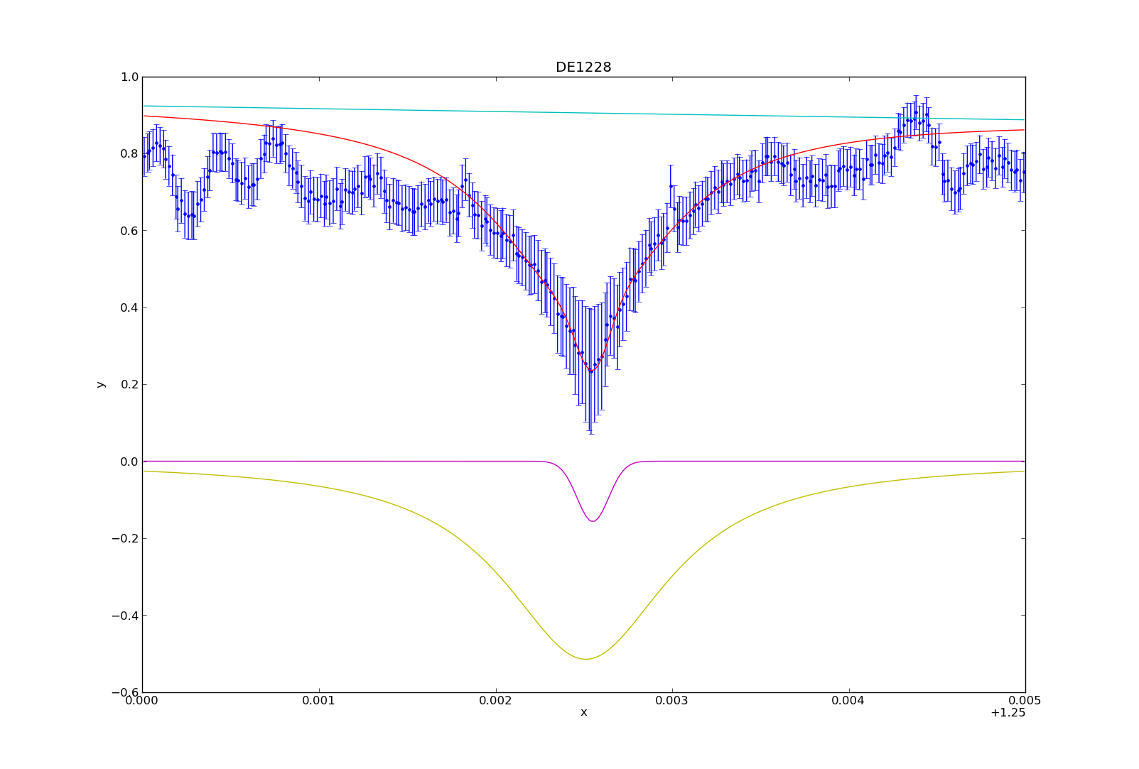
I have spent the last month or so immersing myself in Sherpa, the Python-built program I am using to make the measurements of the Potassium absorption line at 1.2525 microns. While finally coming up for air, I am going to share how I’ve used Sherpa in order to fit a model (or rather, 3 combined models) to the spectral feature so I can make the desired measurements. I will walk you through an example, the plotting and fitting of target “DE1228”.

To start, you need to have all of the data available. Using the BDNYC database developed last semester, we load into arrays the wavelength, flux, and snr values from may 30th, 2007:

>>> w = bdnyc.targets[33].nir[‘high’][‘NIRSPEC’][‘2007may30’][61][‘wl’]
>>> f = bdnyc.targets[33].nir[‘high’][‘NIRSPEC’][‘2007may30’][61][‘flux’]
>>> snr = bdnyc.targets[33].nir[‘high’][‘NIRSPEC’][‘2007may30’][61][‘snr’]

I then used a series of numpy commands to chop the arrays so as to only contain the values from 1.25 to 1.255 microns. Once that was done, I converted the snr to uncertainty values and stored them in an array called “unc”. Since these actions did not require Sherpa, I will omit them from this post. Once I had this completed, it was time to create the Sherpa data structure required for analysis. You use these commands:

>>> from sherpa.astro.ui import *     # This is necessary if you are using Sherpa in a non-standalone version.
>>> data = unpack_arrays(w,f)        # Loads the wavelength and flux arrays into the data structure, which I’ve originally named “data”.
>>> data.name = ‘DE1228’              # Give Sherpa the name of the target — this is not necessary, but it will automatically title any plots from now on.

Now that the data structure is created, we can now start using the sherpa functions to load in the data, models, uncertainties, etc. and bind them to an “id” number. These are the commands I used next:

>>> set_data(1, data)              # I am using the id number “1”, which is the default id number, but I will explicitly state it so you can see how to state it.
>>> set_staterror(1, unc)         # Load in uncertainties as the error
>>> plot_data(1)                      # This plots the data. Error is automatically plotted as well. This is not a necessary step for fitting, but it’s so you can see what you’re dealing with.
>>> set_source(1, powlaw1d.pl+gauss1d.g1+lorentz1d.l1)       # I used a model containing a power law, gaussian profile, and lorentzian profile to fit the data and absorption line.

At this stage in the game, all of the data is now inputted, and now we have to play around. If you want to fit the models to the data, you have to use the fit command:

>>> fit(1)
If you do not prime the program by giving it some good values to start with, it may not come up with anything good. To prime, you can use:
>>> pl.ampl = 9
>>> l1. fwhm  = 0.0011
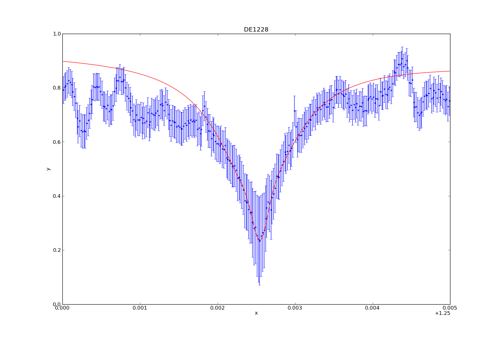
Etcetera. You basically give somewhat good values to start with, and then have it fit the data from there. However, I wanted to fit to the peaks of the continuum data, and the fitting function seemed to be very unstable, often iving me horrible fits even when primed, so I was unable to find a good fit without manually fitting the models to the data myself. For DE1228, I used the values:

>>> pl.gamma = 10
>>> pl.ref = 1
>>> pl.ampl = 8.6
>>> l1.fwhm = 0.00115
>>> l1.pos = 1.25251
>>> l1.ampl = -0.00093
>>> g1.fwhm = 0.00021
>>> g1.pos = 1.25255
>>> g1.ampl = -0.157

Once you’ve fit the model to the data (either manually or not), you can plot the fit by typing:

>>> plot_fit(1)

You can then plot (or overplot) the different model components:

>>> plot_model_component(pl, overplot=True)
>>> plot_model_component(g1, overplot=True)
>>> plot_model_component(l1, overplot=True)

And that’s how I fit the models to the potassium absorption line. I’ve consolidated a lot of these numbers and commands into a table and python module (sherpa_tools.py). While specific, parts of the module can be applied to other people using Sherpa, so I can share the code if needed. In my next blog post, I’ll describe how to utilize the model to make the spectral line measurements (i.e. equivalent width, line-to-continuum flux ratio, full width half maximum).

Sherpa – Week 1 (Plot)

This week, I began to play around with Sherpa, a scientific analysis tool written in Python. Sherpa has two options—you can either run it on its own (aka standalone Sherpa), or you can import it as a Python module, and utilize it in your own scripts. I want to use it for my own purposes, so I’m using it as a module. I’ve been taking notes to use for later documentation on how to use the software to make the spectroscopic measurements mentioned in my previous post.

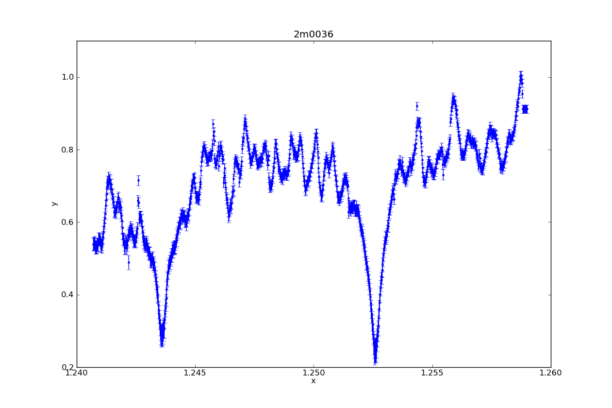
This week, I learned how to take a spectrum (wavelength, flux, and statistical error arrays) and load them into a Sherpa data structure, and then how to plot the spectrum using Sherpa (instead of, say, matplotlib). For the purpose of brevity, I will hand wave these commands and jump to the plots.

Above is a Sherpa plot of one of the L dwarfs in my sample. It is high resolution NIRSPEC data, order 61 (to highlight the Potassium lines). In one easy command (specifically, plot_data), it plotted not only the spectrum, but the statistical error (which I supplied it). It also automatically labeled the axes, and added a title with the name of the target.

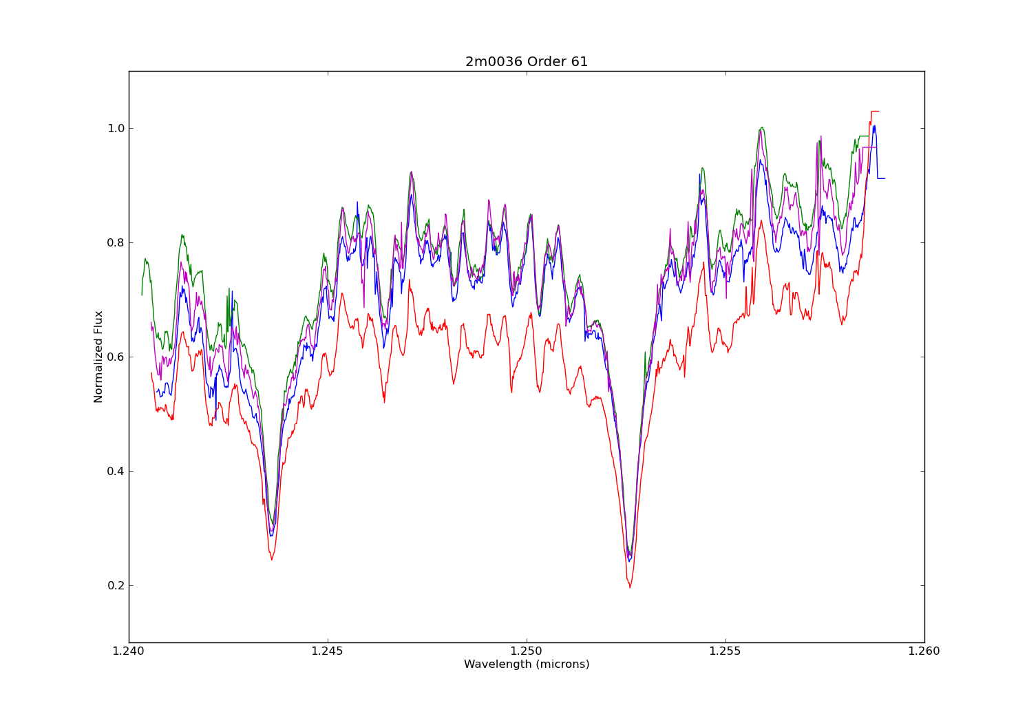
Above is a plot made in matplotlib. I made it not only to make a comparison of the plot styles of the two modules, but also to illustrate the difference between data taken on different nights. Each spectrum plotted here is order 61 from the same target as the Sherpa plot, but observed on different nights (the blue spectrum in this second plot exactly matches that of the first night). Also note that I did not plot the stat. error on the second figure. What stands out for me is that while you can easily notice the jumpiness of the pseudo-continuum, the pseudo-continuum itself is similar on each night. So I think this shows that making a model fit for measuring the potassium features will be roughly the same regardless of the night used.

-Dan