The goal here is to find a prescription of colors diagnostic of brown dwarf surface gravity. Since early optical as well as far infrared spectra and photometry are uncommon, the bands of interest should only include i and z from SDSS; J, H and Ks from 2MASS; and W1, W2 and W3 (but not W4 with only 10 percent detection) from WISE.
In order to find said prescriptions, I used the BT-Settl models (at solar metallicity ranging from 1000 – 3000 K in effective temperature and 3.0 – 5.5 dex in log surface gravity) to produce a suite of color-color and color-parameter plots.
One method I employed was to choose one effective temperature (in this case 2500K) and anchor the colors in one band that doesn’t vary much between high and low surface gravity, e.g. z-band. Then I chose the other two bands by one that was more luminous at low gravity and one that was more luminous at high gravity, e.g. W2- and J-band respectively.
Then the color-color plot of these bands looks like:
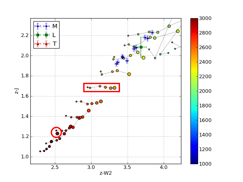
In this plot of z-J vs. z-W2 the smallest circles are objects with high surface gravity and the largest have low surface gravity (log(g) = 5.5 to 3.5 respectively). The light grey lines are iso-temperature contours.
In this particular case, there is little-to-no dispersion in z-J for Teff = 2500K (d = 0.009) and an appreciable dispersion in z-W2 for that same Teff (d = 0.32). Notice the tight vertical grouping (z-J) and dispersed horizontal grouping (z-W2) for the model objects of Teff = 2500K and varying log(g) in the red rectangle on the color-color plot above.
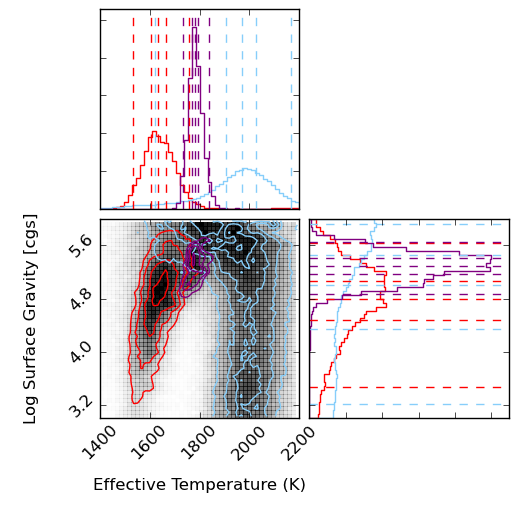
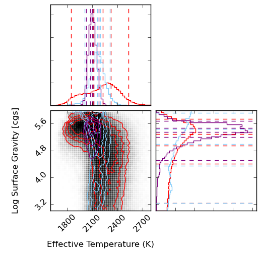
Double-checking with the color-Teff plots, we can see that the dispersion in z-J in the plot on the left is tiny and the horizontal offset in the color-color plot is due to the 0.32 magnitude dispersion in z-W2 on the right below.
-
-
The red box highlights the small dispersion in surface gravity (0.009 mags) at Teff = 2500K.
-
-
The red box highlights the large dispersion in surface gravity (0.32 mags) at Teff = 2500K.
Of course this is just a different way of looking at the same thing, but I might be able to find colors that are reliable indicators of gravity (and thus age) if I can find a bunch of these examples where the flux in the secondary and tertiary bands are flipped.
Of note is the fact that at this temperature in this color-color plot the points are also isolated, i.e. there are no degeneracies with objects of any other temperature. That means that if I find an object with a z-J = 1.65 or so, I know that it has an effective temperature of about 2500K. Then I can determine its age by seeing if its z-W2 color is closer to 3.3 (young) or 2.9 (old).
This of course does not work for all temperatures, as shown in the red circle in the color-color plot above. This demonstrates a degeneracy among hotter young objects (Teff = 3000K, log(g) = 3.5) and cooler old objects (Teff = 2800K, log(g) = 5.5) with a temperature difference of 200K.
Though there is no definitive combination of colors to identify the age of an object irrespective of temperature, what I have done here is found a collection of prescriptions that are reliable indicators of age over small temperature ranges.