Determining ages for brown dwarfs is one of the trickiest aspects in our research, yet a very important one as they allow us to estimate masses. One way many researchers estimate ages is by attempting to match the motions of the object to that of stellar moving groups with known ages. A match in XYZ-UVW space can suggest membership which would imply the brown dwarf is coeval with that group. One can calculate XYZ positions and UVW velocities in Python or your favorite programming language. BDNYC is now hosting a stellar kinematics web application that can do this for you.
Category Archives: Astrometry
Identifying Nearby Young Stars, Part 1: Young Star Isochrones
As stars form, their position on the HR diagram (or, equivalently, a Color-Magnitude diagram) changes. They start out very cool but physically very large and very bright; as they collapse under gravity and become fully supported by hydrogen fusion power, they become smaller and dimmer.
The practical upshot of all of this is that we can determine the ages of stars based on their HR diagram locations – for a given luminosity and color, there is an associated age. This is particularly useful for low-mass objects, which take extremely long times to reach the main sequence: An M0 star probably takes 200 Myr to reach the main sequence (Dotter et al. 2008), while a brown dwarf will never reach any kind of main sequence, and will slowly cool and dim forever.
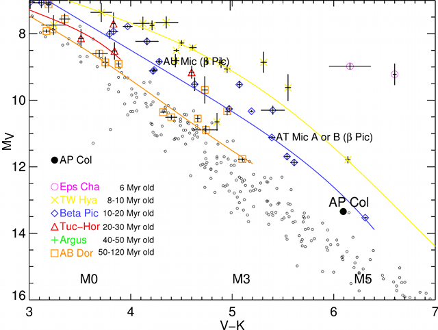
Typically, people use theoretical stellar evolution models like Baraffe et al. (1998), but in practice it is also possible to make empirical relations from known young stars with parallaxes, by fitting polynomials to them. The diagram below shows a set of fifth-order (x5) polynomials that were fit to the single-star members of nearby young associations, as they appeared in Riedel et al. (2011).

A Color-magnitude diagram (Absolute V magnitude versus V-K photometric color) of M dwarf stars with parallaxes. The main sequence is represented by stars with trigonometric (annual) parallaxes within 10 parsecs of the Sun. M dwarf members of associations that are less than ~100 Myr old and closer than 100 parsecs are represented as colored and shaped items on the plot, and empirical isochrones are also shown.
As expected, we see multi-magnitude differences in the luminosity of Epsilon Chameleon members (pink) versus similarly-colored members of TW Hydra (yellow) or Beta Pictoris (blue). On this basis, I presumed the nearby M dwarf AP Columbae was probably older than Beta Pictoris, but younger than AB Doradus (which annoyingly lies within the range of high-metallicity main sequence stars).
Of course, these polynomials are not perfect – they are dependent on the quality of the parallaxes and whether a star actually is a single, “normal” member of the group… and the polynomials are only useful between the boundaries for which there is data to fit. As of the time when I made these polynomial fits, there were only two young brown dwarfs — both members of TW Hydra — with parallaxes AND Johnson V photometry, which is why all the other lines terminate at the middle and hotter M spectral types. If I replaced the Johnson V colors with something redder (I or J-band) it would be a lot easier to produce empirical isochrones for brown dwarfs… although at the moment, extremely few young brown dwarfs are known.
Finding radial velocities
I’ve made good progress on a Python code for finding the radial velocity of an object, and expect it to be done soon! I’m looking forward to finding some radial velocities, and then using the information to determine cluster membership for the brown dwarfs in our sample.
I thought I’d just outline the very basic steps involved in finding radial velocity.
1) Cross correlation: cross correlate two spectra to find how much one is shifted in relation to the other (in pixels). One of these spectra should be a standard for which the radial velocity is known.
2) Convert this shift in pixels to a shift in velocity. Note that this is the velocity with respect to the standard object.
3) Subtract the velocity of the standard from the velocity shift to obtain the radial velocity of your object!
Beginning to find radial velocities for our NIRSPEC data
I’m (for the most part) finished entering our reduced NIRSPEC data into the database. Now I can begin to determine the radial velocities for these objects. In order to find radial velocities, you cross correlate your object’s spectrum with the spectrum of a calibrator whose radial velocity is known. The x-axis “shift” between the two spectra allows you to determine the radial velocity. I’m pretty sure there are a couple of things I need to do before cross-correlating to find the radial velocities (like applying a heliocentric velocity correction to account for our motion around the sun). But we already have a cross correlation code written by another member of our group, and so hopefully things will move pretty quickly from here!
