xtellcor : construct kernel — dealing with missing orders or doublets.

In the help files, you are told that Pa δ contains the least contamination and therefore should be used for constructing the kernel. In cases where this feature shows a doublet, or if you weren’t able to save order 6 (the order that has that particular feature), then you need to use a different feature on another order.

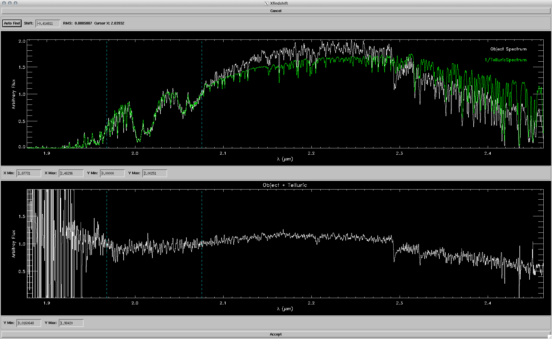
ORDER 5: Generally least contaminated feature is Pa β as shown (Vacca et. al. 2003):

A fit with a polynomial of degree 3 should work just fine (tested on several objects, and data was arguably identical as when done with Pa δ in order 6), and should look a bit like this:

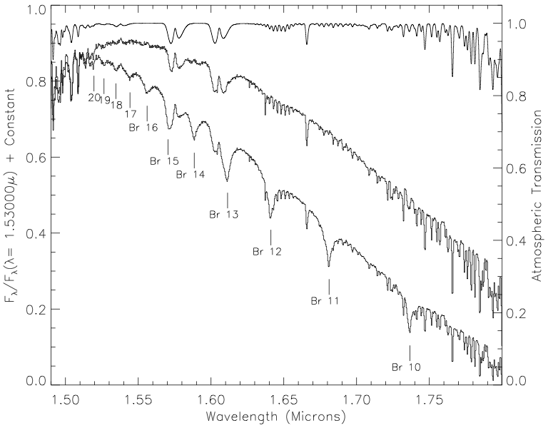
ORDER 4: After a bit of testing, it seems that the best feature here is Br 11, as shown (Vacca et. al. 2003):

A fit with polynomials of degree 2 or 3 should work just fine. If Br 11 has a doublet, please skip it. Doublets are never good.

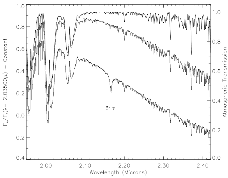
ORDER 3: this order seems to be particularly tricky. At this wavelength, the data starts becoming a bit noisier. The best feature here is Br γ, found at roughly 2.17µ but can often look very contaminated. The majority of the data that I’ve had to deal with have had contamination and therefore it would be wise to not deal with this order unless there are no other options. If order 3 is the only option, then choose Br γ in the location shown below (Vacca et. al. 2003):

This blog post should take care of dealing with construction of spectra. One more point: when normalizing the spectrum, a max deviation around 5% and RMS deviation around 2% is generally acceptable. If max deviation is in the 2% range, and RMS is in the 1% range, then you should expect to produce excellent data.

xtellcor : shifting

>Palomar 200-in, Triple Spectrograph
>Slit: 1×30 arc seconds
>Wavelength coverage: 1.0 – 2.4µ
>Spectral resolution: 2500 – 2700
>Sampling: ~2.7 pixels per resolution element
—————————————————————————————

This is the first blog post of a series of posts detailing some tips and tricks in data reduction of medium resolution brown dwarf spectra (~2500-2700 spectral resolution, ~1.0-2.4µ, 1×30 arcsecond slit) taken from the triple spectrograph at the Palomar 200-in Telescope. The point of this series is to document some easy tips and solutions to small problems for people who are new to the data reduction process using the xSpexTool (Cushing et.al. 2004) and the xTellCor (Vacca et. al. 2003) packages. I’m currently in the process of writing a paper which will serve as a general introduction (targeted for complete beginners) to data reduction. That is soon to come. So let’s start this very brief post about the shifting step of the xtellcor package.

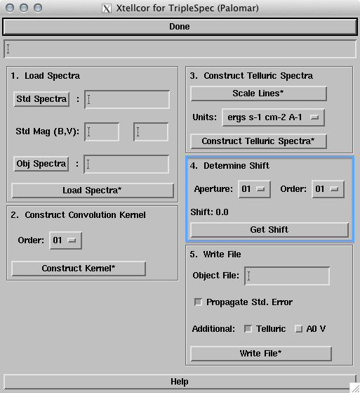
So, you’re at the last step in the xtellcor package:

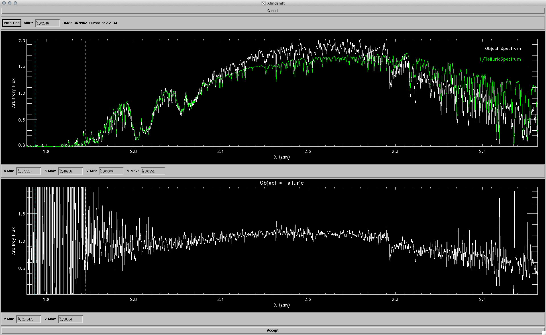
This step is relatively important for medium resolution data. The whole point is for us to output spectra with enough details to distinguish well K, Na, etc. features, but bad shifting can really put a dent on clarity. Let’s use an example. Here we chose object 2m1658+70, with standard SAO 29723. Here is bad shifting (keep in mind, we are not trying hard to get bad data. We just chose a possible area which beginners might also choose):

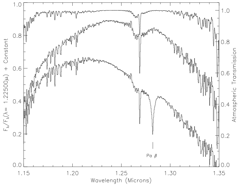
The shift is 1.02. That should automatically start ringing some bells, because although a larger than normal shifting doesn’t necessarily mean it’s bad, it probably means it’s not optimal. Zoom in, and let us compare this shifting with a better one:

The shifting here is -0.41, less than half of the bad one. If you compare the bottom portion of both, you can see that the second one is much less “noisier” on the sides, and generally has clearer, more defined lines. After doing dozens and dozens of objects, it seems that the most optimal areas to select (using “s”) are:

>Order 3 — xMin: 1.965, xMax: 2.075 (roughly -0.40+0.1 shift)
>Order 4 — xMin: 1.455, xMax: 1.535 (roughly -0.30+0.1 shift)
>Order 5 — xMin: 1.180, xMax: 1.245 (roughly -0.45+0.1 shift)
>Order 6 — xMin: 1.100, xMax: 1.165 (roughly -0.20+0.1 shift)

That’s it! Enjoy the data reduction.