Photon Flux Density vs. Energy Flux Density

One of the subtleties of photometry is the difference between magnitudes and colors calculated using energy flux densities (EFD) and photon flux densities (PFD).

The complication arises since the photometry presented by many surveys is calculated using PFD but spectra (specifically the synthetic variety) is given as EFD. The difference is small but measurable so let’s do it right.

The following is the process I used to remedy the situation by switching my models to PFD so they could be directly compared to the photometry from the surveys. Thanks to Mike Cushing for the guidance.

Filter Zero Points

Before we can calculate the magnitudes, we need filter zero points calculated from PFD. To do this, I started with a spectrum of Vega in units of [erg s-1 cm-2 A-1] snatched from STSci.

Then the zero point flux density in [photons s-1 cm-2 A-1] is:

$$!F_{zp}=\frac{\int p_V(\lambda) S(\lambda) d\lambda}{\int S(\lambda)d\lambda}=\frac{\int e_V(\lambda)\left( \frac{\lambda}{hc}\right) S(\lambda) d\lambda}{\int S(\lambda)d\lambda}$$

Where $$e_V$$ is the given energy flux density in [erg s-1 cm-2 A-1] of Vega, $$p_V$$ is the photon flux density in [photons s-1 cm-2 A-1], and $$S(\lambda)$$ is the scalar filter throughput.

Since I’m starting with a spectrum of Vega in EFD units, I need to multiply by $$\frac{\lambda}{hc}$$ to convert it to PFD units.

In Python, this looks like:

def zp_flux(band):
    from scipy import trapz, interp, log10
    (wave, flux), filt, h, c = vega(), get_filters()[band], 6.6260755E-27 # [erg*s], 2.998E14 # [um/s]
    I = interp(wave, filt['wav'], filt['rsr'], left=0, right=0)
    return trapz(I*flux*wave/(h*c), x=wave)/trapz(I, x=wave))

Calculating Magnitudes

Now that we have the filter zero points, we can calculate the magnitudes using:

$$!m = -2.5\log\left(\frac{F_\lambda}{F_{zp}}\right)$$

Where $$m$$ is the apparent magnitude and $$F_\lambda$$ is the flux from our source given similarly by:

$$!F_{\lambda}=\frac{\int p_\lambda(\lambda) S(\lambda) d\lambda}{\int S(\lambda)d\lambda}=\frac{\int e_\lambda(\lambda)\left( \frac{\lambda}{hc}\right) S(\lambda) d\lambda}{\int S(\lambda)d\lambda}$$

Since the synthetic spectra I’m using are given in EFD units, I need to multiply by $$\frac{\lambda}{hc}$$ to convert it to PFD units just as I did with my spectrum of Vega.

In Python the magnitudes are obtained the same way as above but we use the source spectrum in [erg s-1 cm-2 A-1] instead of Vega. Then the magnitude is just:

mag = -2.5*log10(source_flux(band)/zp_flux(band))

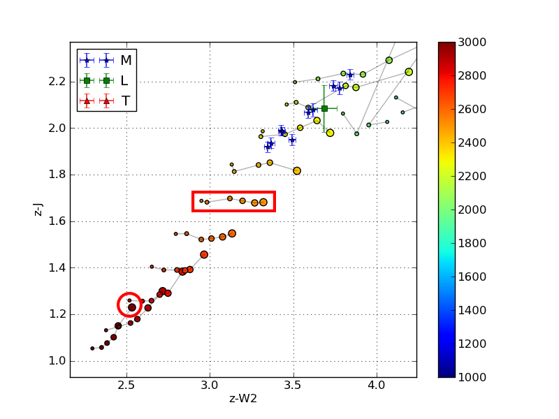
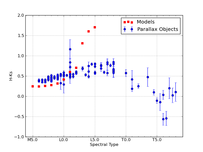
Below is an image that shows the discrepancy between using EFD and PFD to calculate colors for comparison with survey photometry.

The circles are colors calculated from synthetic spectra of low surface gravity (large circles) to high surface gravity (small circles). The grey lines are iso-temperature contours. The jumping shows the different results using PFD and EFD. The stationary blue stars, green squares and red triangles are catalog photometric points calculated from PFD.

The circles are colors calculated from synthetic spectra of low surface gravity (large circles) to high surface gravity (small circles). The grey lines are iso-temperature contours. The jumping shows the different results using PFD and EFD. The stationary blue stars, green squares and red triangles are catalog photometric points calculated from PFD.

Other Considerations

The discrepancy I get between the same color calculated from PFD and EFD though is as much as 0.244 mags (in r-W3 at 1050K), which seems excessive. The magnitude calculation reduces to:

$$!m = -2.5\log\left( \frac{\int e_\lambda(\lambda)S(\lambda) \lambda d\lambda}{\int e_V(\lambda) S(\lambda) \lambda d\lambda}\right)$$

Since the filter profile is interpolated with the spectrum before integration, I thought the discrepancy must be due only to the difference in resolution between the synthetic and Vega spectra. In other words, I have to make sure the wavelength arrays for Vega and the source are identical so the trapezoidal sums have the same width bins.

This reduces the discrepancy in r-W3 at 1050K from -0.244 mags to -0.067 mags, which is better. However, the discrepancy in H-[3.6] goes from 0.071 mags to -0.078 mags.

To Recapitulate

In summary, I had a spectrum of Vega and some synthetic spectra all in energy flux density units of [erg s-1 cm-2 A-1] and some photometric points from the survey catalogs calculated from photon flux density units of [photons s-1 cm-2 A-1].

In order to compare apples to apples, I first converted my spectra to PFD by multiplying by $$\frac{\lambda}{hc}$$ at each wavelength point before integrating to calculate my zero points and magnitudes.

Colors Diagnostic of Surface Gravity

The goal here is to find a prescription of colors diagnostic of brown dwarf surface gravity. Since early optical as well as far infrared spectra and photometry are uncommon, the bands of interest should only include i and z from SDSS; J, H and Ks from 2MASS; and W1, W2 and W3 (but not W4 with only 10 percent detection) from WISE.

In order to find said prescriptions, I used the BT-Settl models (at solar metallicity ranging from 1000 – 3000 K in effective temperature and 3.0 – 5.5 dex in log surface gravity) to produce a suite of color-color and color-parameter plots.

One method I employed was to choose one effective temperature (in this case 2500K) and anchor the colors in one band that doesn’t vary much between high and low surface gravity, e.g. z-band. Then I chose the other two bands by one that was more luminous at low gravity and one that was more luminous at high gravity, e.g. W2- and J-band respectively.

BT-Settl model spectra at 2500K

Then the color-color plot of these bands looks like:

In this plot of z-J vs. z-W2 the smallest circles are objects with high surface gravity and the largest have low surface gravity (log(g) = 5.5 to 3.5 respectively). The light grey lines are iso-temperature contours.

In this plot of z-J vs. z-W2 the smallest circles are objects with high surface gravity and the largest have low surface gravity (log(g) = 5.5 to 3.5 respectively). The light grey lines are iso-temperature contours.

In this particular case, there is little-to-no dispersion in z-J for Teff = 2500K (d = 0.009) and an appreciable dispersion in z-W2 for that same Teff (d = 0.32). Notice the tight vertical grouping (z-J) and dispersed horizontal grouping (z-W2) for the model objects of Teff = 2500K and varying log(g) in the red rectangle on the color-color plot above.

Double-checking with the color-Teff plots, we can see that the dispersion in z-J in the plot on the left is tiny and the horizontal offset in the color-color plot is due to the 0.32 magnitude dispersion in z-W2 on the right below.

Of course this is just a different way of looking at the same thing, but I might be able to find colors that are reliable indicators of gravity (and thus age) if I can find a bunch of these examples where the flux in the secondary and tertiary bands are flipped.

Of note is the fact that at this temperature in this color-color plot the points are also isolated, i.e. there are no degeneracies with objects of any other temperature. That means that if I find an object with a z-J = 1.65 or so, I know that it has an effective temperature of about 2500K. Then I can determine its age by seeing if its z-W2 color is closer to 3.3 (young) or 2.9 (old).

This of course does not work for all temperatures, as shown in the red circle in the color-color plot above. This demonstrates a degeneracy among hotter young objects (Teff = 3000K, log(g) = 3.5) and cooler old objects (Teff = 2800K, log(g) = 5.5) with a temperature difference of 200K.

Though there is no definitive combination of colors to identify the age of an object irrespective of temperature, what I have done here is found a collection of prescriptions that are reliable indicators of age over small temperature ranges.

Color vs. Spectral Type Model Comparison

Here are color vs. spectral type plots for the 2MASS J, H and Ks bands.

The blue circles are for the objects with parallax measurements. The red squares are for the AMES-Dusty model spectra with spectral types gleaned from effective temperature according to Golimowski et al (2004).

While the AMES-Dusty models are known not to be a good fit for objects with effective temperatures lower than about 2200K (shown by the disagreement in L dwarf colors of objects and models), the M dwarfs fit fairly well for J-Ks versus Spectral Type.

However, the models are under-luminous in J-H and over-luminous in H-Ks for M dwarfs, indicating a possible problem with H-band modeling. The models shown are calculated with a surface gravity of 5.5, which means that the models produce a “peakier” H-band than the objects actually exhibit.

In a color-color plot of J-H versus H-Ks, the H-band throws off the model colors on both axes causing a diagonal shift (bluer in J-H, redder in H-Ks) of M and L dwarfs compared to the models:

Spectral Energy Distributions

The goal here was to investigate the atmospheric properties of known young objects and identify new brown dwarf candidates by producing extended spectral energy distributions (SEDs).

These SEDs are constructed by combining WISE mid-infrared photometry with our extensive database of optical and near-infrared spectra and parallaxes. The BDNYC Database has about 875 objects and the number of objects with parallaxes is about 250.

My code queries the database and the parallax measurements by right ascension and declination and then identifies the matches with enough spectra and photometry to produce an SED. Next, it checks the flux and wavelength units and makes the appropriate conversions to [ergs][s-1][cm-2][cm-1] and [um] respectively.

It then runs a fitting routine across BT-Settl models of every permutation of:

  • 400 K < Teff < 4500 K in 50 K increments,
  • 3.0 dex < log(g) < 5.5 dex in 0.1 dex increments, and
  • 0.5 MJup < radius < 1.3 MJup in 0.05 MJup increments.

Once the best match is found, it plots the synthetic spectrum (grey) along with the photometric points converted to flux in each SDSS, 2MASS and WISE bands (grey dots). In this manner, the fitting routine guesses the effective temperature, surface gravity and radius simultaneously.

Here are some preliminary plots:

Converting Between Decimal Degrees and Hours, Minutes, Seconds

Here’s a quick Python snippet I wrote to convert right ascension in decimal degrees to hours, minutes, seconds and declination to (+/-)degrees, minutes, seconds.

def deg2HMS(ra='', dec='', round=False):
  RA, DEC, rs, ds = '', '', '', ''
  if dec:
    if str(dec)[0] == '-':
      ds, dec = '-', abs(dec)
    deg = int(dec)
    decM = abs(int((dec-deg)*60))
    if round:
      decS = int((abs((dec-deg)*60)-decM)*60)
    else:
      decS = (abs((dec-deg)*60)-decM)*60
    DEC = '{0}{1} {2} {3}'.format(ds, deg, decM, decS)
  
  if ra:
    if str(ra)[0] == '-':
      rs, ra = '-', abs(ra)
    raH = int(ra/15)
    raM = int(((ra/15)-raH)*60)
    if round:
      raS = int(((((ra/15)-raH)*60)-raM)*60)
    else:
      raS = ((((ra/15)-raH)*60)-raM)*60
    RA = '{0}{1} {2} {3}'.format(rs, raH, raM, raS)
  
  if ra and dec:
    return (RA, DEC)
  else:
    return RA or DEC

For example:
In [1]: f.deg2HMS(ra=66.918277)
Out[1]: '4 27 40.386'

Or even:
In [2]: f.deg2HMS(dec=24.622590)
Out[2]: '+24 37 21.324'

Or if you want to round the seconds, just do:
In [3]: f.deg2HMS(dec=24.622590,round=True)
Out[3]: '+24 37 21'

And to convert hours, minutes and seconds into decimal degrees, we have:

def HMS2deg(ra='', dec=''):
  RA, DEC, rs, ds = '', '', 1, 1
  if dec:
    D, M, S = [float(i) for i in dec.split()]
    if str(D)[0] == '-':
      ds, D = -1, abs(D)
    deg = D + (M/60) + (S/3600)
    DEC = '{0}'.format(deg*ds)
  
  if ra:
    H, M, S = [float(i) for i in ra.split()]
    if str(H)[0] == '-':
      rs, H = -1, abs(H)
    deg = (H*15) + (M/4) + (S/240)
    RA = '{0}'.format(deg*rs)
  
  if ra and dec:
    return (RA, DEC)
  else:
    return RA or DEC

So we can get back our decimal degrees with:

In [4]: f.HMS2deg(ra='4 27 40.386', dec='+24 37 21.324')
Out[4]: (66.918, 24.622)

How to Make Animated GIFs of Plots

So you’re swimming in countless plots of your data over some changing parameter. Sure they’re nice to look at, but are they animated? Didn’t think so.

Here’s how to create an animated .gif image of those Python plots using Photoshop.

Step 1: Generate the plots

I’ve found that a few lines of Python to programmatically draw and save your plots to a folder eliminates a lot of editing and tweaking later on.

For this tutorial, I’ll use my synthetic photometry code to generate color-parameter plots across surface gravities of 3.0dex to 6.0dex.

First I created a folder on my desktop to dump the plots called RI_teff.

Then in the Python interpreter it looks like:

In [1]: grav = [round(i*0.1,1) for i in range(30,61)]
In [2]: import syn_phot as s
In [3]: for i in g:
s.color_param('R','I',logg=i,save='/Desktop/RI_teff/')

Now I can create the animated .gif in Photoshop.

Step 2: Pull plots into Photoshop as layers

Open Photoshop and click File > Scripts > Load Files into Stack…

Select the folder on your Desktop that has all the plots and click ok.

Photoshop will open each image as a layer in a new project window.

Step 3: Create frames from each layer

Next click Window > Timeline to show the Timeline across the bottom of the program.

In the top-right corner of your Timeline, you’ll see a little button that has all the Timeline options. Click it and select Make Frames From Layers. Here’s what it looks like:

This will populate your Timeline with one frame for each image layer.

Click the Timeline options button again and click Reverse Frames if necessary. Otherwise, you can drag and drop the frames into the desired order.

Step 4: Timing is everything

Next we need to set the timing of each frame. Select the first frame from the Timeline then hold down the Shift button and select the last frame to select them all.

Next click on any frame where it says 0 sec. with a down arrow. Then select the display time for each frame in the animation.

I typically set the frames to be 0.2 or 0.5 seconds each, depending on the number of total frames. Then I set the last frame to be 2 seconds so it’s as if the image pauses when it finishes before starting the animation over.

Step 5: Save it!

Finally, click File > Save for Web… and make sure you have GIF filetype selected. Click Save and you’re done! Here’s the result:

Editing PYTHONPATH (or “Where’s my module?!”)

Python not finding your modules with import MyModule for some reason? It’s probably your PYTHONPATH. Here’s how you edit it so that Python sees all your modules.

A Word About Directories

Firstly, if you are the kind of person who keeps files scattered about your computer, dumps everything into the root directory, or is afraid to use those nice little blue folders, then perhaps programming and computers in general are not for you.

Logical and neat directory structure will make your own, your computer’s and your collaborators’ lives much easier.

My recommendation: Create a master code directory (called “Modules” or something) in your Documents folder. This will be the new home of all your future Python projects.

Now every time you create a .py file, it should go into a project folder inside your Modules directory, i.e. /Documents/Modules/NewProject/MyModule.py. Note that you should have no actual modules inside your Modules directory! Keep those puppies in their warm, snuggly project subdirectories.

This way you can also initialize that project folder (i.e. /NewProject) as a Git repository and just push and pull the contents to keep it up-to-date!

Editing PYTHONPATH

Python won’t just search your computer for the MyModule.py file you’re trying to import. You have to tell it explicitly each time where to get it. The PYTHONPATH is a list of directories for your computer to check whenever you type import MyModule into the interpreter.

To add a path, launch ipython and type:

import sys
sys.path.append("path/to/Modules")
print sys.path

Note: You only have to update your PYTHONPATH once, not every time you use Python!

So now your path is updated but this is only the path to your master Python folder.

In order to have Python see the modules inside each subdirectory, add a blank file called __init__.py to each subdirectory (with two underscores on each side).

Now to import the module and use a function called foo() do:

from NewProject import MyModule as m
m.foo()

That is, it’s checking the main python directory you added to your PYTHONPATH, then looking within the NewProject subdirectory via the __init__.py file for the module you’re trying to import.

Brown Dwarf Synthetic Photometry

The goal here was to get the synthetic colors in the SDSS, 2MASS and WISE filters of ~2000 model objects generated by the PHOENIX stellar and planetary atmosphere software.

Since it would be silly (and incredibly slow… and much more boring) to just calculate and store every single color for all 12 filter profiles, I wrote a module to calculate colors a la carte.

The Filters

I got the J, H, and K band relative spectral response (RSR) curves in the 2MASS documentation, the u, g, r, i and z bands from the SDSS documentation, and the W1, W2, W3, and W4 bands from the WISE documentation.

I dumped all my .txt filter files into one directory and wrote a function to grab them all, pull out the wavelength and transmission values, and output the filter name in position [0], x-values in [1], and y-values in [2]:

def get_filters(filter_directory):
  import glob, os
  files = glob.glob(filter_directory+'*.txt')
 
  if len(files) == 0:
    print 'No filters in', filter_directory
  else:
    filter_names = [os.path.splitext(os.path.basename(i))[0] for i in files]
    RSR = [open(i) for i in files]
    filt_data = [filter(None,[map(float,i.split()) for i in j if not i.startswith('#')]) for j in RSR]
    for i in RSR: i.close()
 
    RSR_x = [[x[0] for x in i] for i in filt_data]
    RSR_y = [[y[1] for y in i] for i in filt_data]
    filters = {}
    for i,j,k in zip(filter_names,RSR_x,RSR_y):
      filters[i] = j, k, center(i)
 
    return filters

Calculating Apparent Magnitudes

We can’t have colors without magnitudes so here’s a function to grab the Teff and log g specified spectra, and calculate the apparent magnitudes in a particular band:

def mags(band, teff='', logg='', bin=1):
  from scipy.io.idl import readsav
  from collections import Counter
  from scipy import trapz, log10, interp
  
  s = readsav(path+'modelspeclowresdustywise.save')
  Fr, Wr = [i for i in s.modelspec['fsyn']], [i for i in s['wsyn']]
  Tr, Gr = [int(i) for i in s.modelspec['teff']], [round(i,1) for i in s.modelspec['logg']]
  
  # The band to compute
  RSR_x, RSR_y, lambda_eff = get_filters(path)[band]
  
  # Option to specify an effective temperature value
  if teff:
    t = [i for i, x in enumerate(s.modelspec['teff']) if x == teff]
    if len(t) == 0:
      print "No such effective temperature! Please choose from 1400K to 4500K in 50K increments or leave blank to select all."
  else:
    t = range(len(s.modelspec['teff']))
  
  # Option to specify a surfave gravity value
  if logg:
    g = [i for i, x in enumerate(s.modelspec['logg']) if x == logg]
    if len(g) == 0:
      print "No such surface gravity! Please choose from 3.0 to 6.0 in 0.1 increments or leave blank to select all."
  else:
    g = range(len(s.modelspec['logg']))
  
  # Pulls out objects that fit criteria above
  obj = list((Counter(t) & Counter(g)).elements())
  F = [Fr[i][::bin] for i in obj]
  T = [Tr[i] for i in obj]
  G = [Gr[i] for i in obj]
  W = Wr[::bin]
  
  # Interpolate to find new filter y-values
  I = interp(W,RSR_x,RSR_y,left=0,right=0)
  
  # Convolve the interpolated flux with each filter (FxR = RxF)
  FxR = [convolution(i,I) for i in F]
  
  # Integral of RSR curve over all lambda
  R0 = trapz(I,x=W)
  
  # Integrate to find the spectral flux density per unit wavelength [ergs][s-1][cm-2] then divide by R0 to get [erg][s-1][cm-2][cm-1]
  F_lambda = [trapz(y,x=W)/R0 for y in FxR]
  
  # Calculate apparent magnitude of each spectrum in each filter band
  Mags = [round(-2.5*log10(m/F_lambda_0(band)),3) for m in F_lambda]
  
  result = sorted(zip(Mags, T, G, F, I, FxR), key=itemgetter(1,2))
  result.insert(0,W)
  
  return result

Calculating Colors

Now we can calculate the colors. Next, I wrote a function to accept any two bands with options to specify a surface gravity and/or effective temperature as well as a bin size to cut down on computation. Here’s the code:

def colors(first, second, teff='', logg='', bin=1):
  (Mags_a, T, G) = [[i[j] for i in get_mags(first, teff=teff, logg=logg, bin=bin)[1:]] for j in range(3)]
  Mags_b = [i[0] for i in get_mags(second, teff=teff, logg=logg, bin=bin)[1:]]
  colors = [round(a-b,3) for a,b in zip(Mags_a,Mags_b)]
  
  print_mags(first, colors, T, G, second=second)
  
  return [colors, T, G]

The PHOENIX code gives the flux as Fλ in cgs units [erg][s-1][cm-2][cm-1] but as long as both spectra are in the same units the colors will be the same.

Makin’ It Handsome

Then I wrote a short function to print out the magnitudes or colors in the Terminal:

def print_mags(first, Mags, T, G, second=''):
  LAYOUT = "{!s:10} {!s:10} {!s:25}"
  
  if second:
    print LAYOUT.format("Teff", "log g", first+'-'+second)
  else:
    print LAYOUT.format("Teff", "log g", first)
  
  for i,j,k in sorted(zip(T, G, Mags)):
    print LAYOUT.format(i, j, k)

The Output

Then if I just want the J-K color for objects with log g = 4.0 over the entire range of effective temperatures, I launch ipython and just do:

In [1]: import syn_phot as s
In [2]: s.colors('J','K', logg=4)
Teff -------- log g -------- J-K
1400.0 ------ 4.0 ---------- 4.386
1450.0 ------ 4.0 ---------- 4.154
...
4450.0 ------ 4.0 ---------- 0.756
4500.0 ------ 4.0 ---------- 0.733

Similarly, I can specify just the target effective temperature and get the whole range of surface gravities. Or I can specify an effective temperature AND a specific gravity to get the color of just that one object with:

In [3]: s.colors('i','W2', teff=3050, logg=5)
Teff -------- log g -------- J-K
3050.0 ------ 5.0 ---------- 3.442

I can also reduce the number of data points in each flux array if my sample is very large. I just have to specify the number of data points to skip with the “bin” optional parameter. For example:

In [4]: s.colors('W1','W2', teff=1850, bin=3)

This will calculate the W1-W2 color for all the objects with Teff = 1850K and all gravities, but only take every third flux value.

I also wrote functions to generate color-color, color-parameter and color-magnitude plots but those will be in a different post.

Plots!

Here are a few color-parameter animated plots I made using my code. Here’s how I made them. Click to animate!

And here are a few colorful-colorful color-color plots I made:

Plots with observational data

Just to be sure I’m on base, here’s a color-color plot of J-H vs. H-Ks for objects with a log surface gravity of 5 dex (blue dots) plotted over some data for the Chamaeleon I Molecular Cloud (semi-transparent) from Carpenter et al. (2002).

The color scale is for main sequence stars and the black dots are probable members of the group. Cooler dwarfs move up and to the right.

And here’s a plot of J-Ks vs. z-Ks as well as J-Ks vs. z-J. Again, the blue dots are from my synthetic photometry code at log(g)=5 and the semi-transparent points with errors are from Dahn et al. (2002).