Creating a Database with astrodbkit

NOTE: The information on this post may be outdated. We recommend looking into the up-to-date documentation at trac (internal) and ReadTheDocs.

The astrodbkit package can be used to modify an existing SQL database (such as The BDNYC Database) but it can also be used to create and populate a SQL database from scratch.

To do this, import the BDdb module and create a new database with
from astrodbkit import astrodb
dbpath = '/path/to/new_database.db'
astrodb.create_databse(dbpath)

Then load your new database with

db = astrodb.Database(dbpath)

and start adding tables! The db.table() method accepts as its arguments the table name, list of field names, and list of data types like so:

db.table('my_new_table', ['field1','field2'], ['INTEGER','TEXT'], new_table=True)

Note new_table=True is necessary to create a new table. Otherwise, it looks for an existing table to modify (which you could do as well!).

To populate your new database with data, read the documentation here or a summary at Adding Data to the BDNYC Database.

As always, I recommend the SQLite Browser for a nice GUI to make changes outside of the command line.

Happy databasing!

Updating the astrodbkit documentation

As you make changes to the astrodbkit repository on Github, you may find that the documentation needs updating. Luckily, we use the invaluable Sphinx and the awesome ReadTheDocs to generate the documentation so this is fairly simple.

First, make sure you update the appropriate doc strings (those informative green bits just below the function definition) as this is what Sphinx will use to generate the documentation!

Start in the top level astrodbkit directory and generate the documentation from the module docstrings with

sphinx-build docs astrodbkit -a

Then cd into the docs directory and rebuild the html files with

cd docs
make html

Now move back to the top level directory and add, commit, and push your changes to Github with something like

cd ..
git add /docs
git commit -m "Updated the documentation for methods x, y, and z."
git push origin <your_branch>

All set! Refresh the page (after a few minutes so ReadTheDocs can build the pages) and make sure everything is to your liking. Well done.

And just in case, here’s a great tutorial for getting started with Sphinx and here’s the official documentation.

Deploying Package Releases to PyPI

Registering the package

To register the package and deploy the initial release to PyPI, do:

python setup.py register -r pypi
python setup.py sdist upload -r pypi

Deploying a new release

So you’ve made some cool new improvements to your Python package and you want to deploy a new release. It’s just a few easy steps.

  1. After your package modules have been updated, you have to update the version number in your setup.py file. The format is major.minor.micro depending on what you changed. For example, a small bug fix to v0.2.3 would increment to v0.2.4 while a new feature might increment to v0.3.0.
  2. Then make sure all the changes are committed and pushed to Github.
  3. Build with python setup.py sdist
  4. Twine with twine upload dist/compressed_package_filename

That’s it!

Adding Data to a SQL Database using astrodbkit

NOTE: The information on this post may be outdated. We recommend looking into the up-to-date documentation at trac (internal) and ReadTheDocs.

To add data to any table, there are two easy steps. As our working example, we’ll add some new objects to the SOURCES table.

Step 1: Create an ascii file of the data

First, you must choose a delimiter, which is just the character that will break up the data into columns. I recommend a pipe ‘|’ character since they don’t normally appear in text. This is better than a comma since some data fields may have comma-separated values.

Put the data to be added in an ascii file with the following formatting:

  1. The first line must be the |-separated column names to insert/update, e.g. ra|dec|publication_id. Note that the column names in the ascii file need not be in the same order as the table. Also, only the column names that match will be added and non-matching or missing column names will be ignored, e.g. spectral_type|ra|publication_id|dec will ignore the spectral_type values as this is not a column in the SOURCES table and input the other columns in the correct places.
  2. If a record (i.e. a line in your ascii file) has no value for a particular column, type nothing. E.g. for the given column names ra|dec|publication_id|comments, a record with no publication_id should read 34.567|12.834||This object is my favorite!.

Step 2: Add the data to the specified table

To add the data to the table (in our example, the SOURCES table), import astrodbkit and initialize the .db file. Then run the add_data() method with the path to the ascii file as the first argument and the table to add the data to as the second argument. Be sure to specify your delimiter with delim='|'. Here’s what that looks like:

from astrodbkit import astrodb
db = astrodb.Database('/path/to/the/database/file.db')
db.add_data('/path/to/the/upload/file.csv', 'sources', delim='|')

That’s it!

Uncertainty Propagation

All observations have associated uncertainties which must be propagated through your analysis to a an uncertainty on a final result. The principle of uncertainty propagation is fairly simple:

$$!\sigma_x^2 = \sigma_u^2\left(\frac{\partial x}{\partial u}\right)^2 + \sigma_v^2\left(\frac{\partial x}{\partial v}\right)^2+\dots +2\sigma_{uv}^2\left(\frac{\partial x}{\partial u}\right)\left(\frac{\partial x}{\partial v}\right)+\dots$$

The first two terms on the right are the averages of the squares of the deviations in x produced by the uncertainties in observables u and v respectively. The third term on the right is the average of the cross terms, which cancel out if u and v are uncorrelated. Thus in most situations, a reasonable approximation is:

$$!\sigma_x^2 = \sum\limits_u\sigma_u^2\left(\frac{\partial x}{\partial u}\right)^2$$

Examples

A typical situation is the sum of two observables each with a multiplicative factor:

$$!x=au+bv$$

$$!\left(\frac{\partial x}{\partial u}\right)=a,\hspace{10pt}\left(\frac{\partial x}{\partial v}\right)=b$$

$$!\sigma_x = \sqrt{\sigma_u^2a^2 + \sigma_v^2b^2}$$

which is the oft used “summing in quadrature.”

Perhaps you have the product of two observables:

$$!x=auv+b$$

$$!\left(\frac{\partial x}{\partial u}\right)=av,\hspace{10pt}\left(\frac{\partial x}{\partial v}\right)=au$$

$$!\sigma_x = \sqrt{\sigma_u^2(av)^2 + \sigma_v^2(au)^2}=a\sqrt{\sigma_u^2v^2 + \sigma_v^2u^2}$$

Finally, perhaps you have the inverse of one observable times the exponential of another:

$$!x=\frac{a}{u}e^{bv}$$

$$!\left(\frac{\partial x}{\partial u}\right)=\left(-\frac{a}{u^2}\right)e^{bv},\hspace{10pt}\left(\frac{\partial x}{\partial v}\right)=\frac{a}{u}be^{bv}$$

$$!\sigma_x = \sqrt{\sigma_u^2\left(\frac{a}{u^2}e^{bv}\right)^2 + \sigma_v^2\left(\frac{a}{u}be^{bv}\right)^2}=\frac{a}{u}e^{bv}\sqrt{\frac{\sigma_u^2}{u^2}+\sigma_v^2b^2}$$

Easy!

Setting Up Your BDNYC Astro Python Environment

Here’s a step-by-step tutorial on how to set up your Python development environment.

Distribution and Compiler

The first step is to install Anaconda. Click here, select the appropriate version for your machine and operating system, download the .dmg file, open it and double-click the installer.

Make sure that when the installer asks where to put the distribution, you choose your actual hard drive and not some sub-directory on your machine. This will make things much easier later on.

What’s nice about this distribution is that it includes common plotting, computing, and astronomy packages such as numpy and scipy, astropy, matplotlib, and many others.

Next you’ll need a C compiler. If you’re using MacOSX, I recommend using Xcode which you can download free here. (This step may take a while so go get a beverage.) Once the download is complete, run the installer.

Required Packages

For future installation of packages, I recommend using Pip. To install this, at your Terminal command line type sudo easy_install pip. Then whenever you want to install a package you might need, you just open Terminal and do pip install package_name.

Not every package is this easy (though most are). If you can’t get something through Pip just download, unzip and put the folder of your new module with the rest of your packages in the directory /anaconda/pkgs/.

Then in Terminal, navigate to that directory with cd /anaconda/pkgs/package_dir_name and do python setup.py install.

Development Tools

MacOSX comes with the text editing application TextEdit but it is not good for editing code. I strongly recommend using TextMate though it is not free so you should ask your advisor to buy a license for you! Otherwise, some folks find the free TextWrangler to be pretty good.

Next, you’ll want to get access to the BDNYC database. Detailed instructions are here on how to setup Dropbox and Github on your machine in order to interact with the database.

Launching Python

Now to use Python, in Terminal just type ipython --pylab. I recommend always launching Python this way to have the plotting library preloaded.

Enjoy!

BDNYC Database Setup

WARNING: The information on this is outdated. We recommend looking into the up-to-date documentation at trac (internal) and ReadTheDocs.

Read this post first if your development environment needs setting up. Then…

Setting Up the Database

To install the database, open a Terminal session and do:

pip install BDNYCdb

Then download the public database file BDNCY198.db here or get the unpublished BDNYC.db file from Dropbox. (Ask a group member for the invite!)

Accessing the Database

Now you can load the entire database into a Python variable simply by launching the Python interpreter and pointing the get_db() function to the database file by doing:

In [1]: from BDNYCdb import BDdb
In [2]: db = BDdb.get_db('/path/to/your/Dropbox/BDNYCdb/BDNYC.db')

Voila!

In the database, each source has a unique identifier (or ‘primary key’ in SQL speak). To see an inventory of all data for one of these sources, just do:

In [3]: db.inventory(id)

where id is the source_id.

Now that you have the database at your fingertips, you’ll want to get some info out of it. To do this, you can use SQL queries.

Here is a detailed post about how to write an SQL query.

Further documentation for sqlite3 can be found here. Most commands involve wrapping SQL language inside python functions. The main method we will use to fetch data from the database is list():

In [5]: data = db.list( "SQL_query_goes_here" ).fetchall()

Example Queries

Some SQL query examples to put in the command above (wrapped in quotes of course):

  1. SELECT shortname, ra, dec FROM sources WHERE (222<ra AND ra<232) AND (5<dec AND dec<15)
  2. SELECT band, magnitude, magnitude_unc FROM photometry WHERE source_id=58
  3. SELECT source_id, band, magnitude FROM photometry WHERE band=’z’ AND magnitude<15
  4. SELECT wavelength, flux, unc FROM spectra WHERE observation_id=75”

As you hopefully gathered:

  1. Returns the shortname, ra and dec of all objects in a 10 square degree patch of sky centered at RA = 227, DEC = 10
  2. Returns all the photometry and uncertainties available for object 58
  3. Returns all objects and z magnitudes with z less than 15
  4. Returns the wavelength, flux and uncertainty arrays for all spectra of object 75

The above examples are for querying individual tables only. We can query from multiple tables at the same time with the JOIN command like so:

  1. SELECT t.name, p.band, p.magnitude, p.magnitude_unc FROM telescopes as t JOIN photometry AS p ON p.telescope_id=t.id WHERE p.source_id=58
  2. SELECT p1.magnitude-p2.magnitude FROM photometry AS p1 JOIN photometry AS p2 ON p1.source_id=p2.source_id WHERE p1.band=’J’ AND p2.band=’H’
  3. SELECT src.designation, src.unum, spt.spectral_type FROM sources AS src JOIN spectral_types AS spt ON spt.source_id=src.id WHERE spt.spectral_type>=10 AND spt.spectral_type<20 AND spt.regime=’optical’
  4. SELECT s.unum, p.parallax, p.parallax_unc, p.publication_id FROM sources as s JOIN parallaxes AS p ON p.source_id=s.id

As you may have gathered:

  1. Returns the survey, band and magnitude for all photometry of source 58
  2. Returns the J-H color for every object
  3. Returns the designation, U-number and optical spectral type for all L dwarfs
  4. Returns the parallax measurements and publications for all sources

Alternative Output

As shown above, the result of a SQL query is typically a list of tuples where we can use the indices to print the values. For example, this source’s g-band magnitude:

In [9]: data = db.list("SELECT band,magnitude FROM photometry WHERE source_id=58").fetchall()
In [10]: data
Out[10]: [('u', 25.70623),('g', 25.54734),('r', 23.514),('i', 21.20863),('z', 18.0104)]
In [11]: data[1][1]
Out[11]: 25.54734

However we can also query the database a little bit differently so that the fields and records are returned as a dictionary. Instead of db.query.execute() we can do db.dict() like this:

In [12]: data = db.dict("SELECT * FROM photometry WHERE source_id=58").fetchall()
In [13]: data
Out[13]: [<sqlite3.Row at 0x107798450>, <sqlite3.Row at 0x107798410>, <sqlite3.Row at 0x107798430>, <sqlite3.Row at 0x1077983d0>, <sqlite3.Row at 0x1077982f0>]
In [14]: data[1]['magnitude']
Out[14]: 25.54734

Database Schema and Browsing

In order to write the SQL queries above you of course need to know what the names of the tables and fields in the database are. One way to do this is:

In [15]: db.list("SELECT sql FROM sqlite_master").fetchall()

This will print a list of each table, the possible fields, and the data type (e.g. TEXT, INTEGER, ARRAY) for that field.

SQL browserEven easier is to use the DB Browser for SQLite pictured at left which lets you expand and collapse each table, sort and order columns, and other fun stuff.

It even allows you to manually create/edit/destroy records with a very nice GUI.

IMPORTANT: If you are using the private database keep in mind that if you change a database record, you immediately change it for everyone since we share the same database file on Dropbox. Be careful!

Always check and double-check that you are entering the correct data for the correct source before you save any changes with the SQLite Database Browser.

SQL Queries

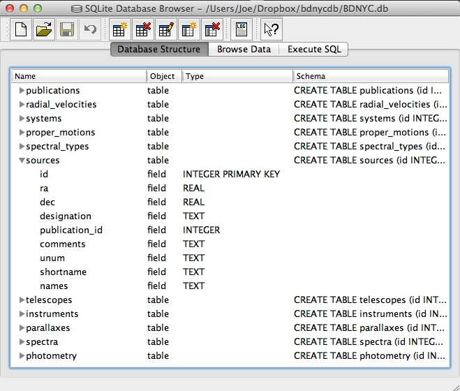
An SQL database is comprised of a bunch of tables (kind of like a spreadsheet) that have fields (column names) and records (rows of data). For example, our database might have a table called students that looks like this:

id first last grade GPA
1 Al Einstein 6 2.7
2 Annie Cannon 6 3.8
3 Artie Eddington 8 3.2
4 Carlie Herschel 8 3.2

So in our students table, the fields are [id, first, last, grade, GPA], and there are a total of four records, each with a required yet arbitrary id in the first column.

To pull these records out, we tell SQL to SELECT values for the following fields FROM a certain table. In SQL this looks like:

In [1]: db.execute("SELECT id, first, last, grade, GPA FROM students").fetchall()
Out[1]: [(1,'Al','Einstein',6,2.7),(2,'Annie','Cannon',6,3.8),(3,'Artie','Eddington',8,3.2),(4,'Carlie','Herschel',8,3.2)]

Or equivalently, we can just use a wildcard “*” if we want to return all fields with the SQL query "SELECT * FROM students".

We can modify our SQL query to change the order of fields or only return certain ones as well. For example:

In [2]: db.execute("SELECT last, first, GPA FROM students").fetchall()
Out[1]: [('Einstein','Al',2.7),('Cannon','Annie',3.8),('Eddington','Artie',3.2),('Herschel','Carlie',3.2)]

Now that we know how to get records from tables, we can restrict which records it returns with the WHERE statement:

In [3]: db.execute("SELECT last, first, GPA FROM students WHERE GPA>3.1").fetchall()
Out[3]: [('Cannon','Annie',3.8),('Eddington','Artie',3.2),('Herschel','Carlie',3.2)]

Notice the first student had a GPA less than 3.1 so he was omitted from the result.

Now let’s say we have a second table called quizzes which is a table of every quiz grade for all students that looks like this:

id student_id quiz_number score
1 1 3 89
2 2 3 96
3 3 3 94
4 4 3 92
5 1 4 78
6 3 4 88
7 4 4 91

Now if we want to see only Al’s grades, we have to JOIN the tables ON some condition. In this case, we want to tell SQL that the student_id (not the id) in the quizzes table should match the id in the students table (since only those grades are Al’s). This looks like:

In [4]: db.execute("SELECT quizzes.quiz_number, quizzes.score FROM quizzes JOIN students ON students.id=quizzes.student_id WHERE students.last='Einstein'").fetchall()
Out[4]: [(3,89),(4,78)]

So students.id=quizzes.student_id associates each quiz with a student from the students table and students.last='Einstein' specifies that we only want the grades from the student with last name Einstein.

Similarly, we can see who scored 90 or greater on which quiz with:

In [5]: db.execute("SELECT students.last, quizzes.quiz_number, quizzes.score FROM quizzes JOIN students ON students.id=quizzes.student_id WHERE quizzes.score>=90").fetchall()
Out[5]: [('Cannon',3,96),('Eddington',3,94),('Herschel',3,92),('Herschel',4,91)]

That’s it! We can JOIN as many tables as we want with as many restrictions we need to pull out data in the desired form.

This is powerful, but the queries can become lengthy. A slight shortcut is to use the AS statement to assign a table to a variable (e.g. students => s, quizzes => q) like such:

In [6]: db.execute("SELECT s.last, q.quiz_number, q.score FROM quizzes AS q JOIN students AS s ON s.id=q.student_id WHERE q.score>=90").fetchall()
Out[6]: [('Cannon',3,96),('Eddington',3,94),('Herschel',3,92),('Herschel',4,91)]

Ground Based Photometry

Here I want to calculate some photometric points from spectra for comparison with published values for a bunch of known brown dwarfs.

In order to get the true magnitude $$m$$ for an object, I first need to calculate the instrumental magnitude $$m_\text{inst}$$ and then correct for a number of effects. That is, I calculate the apparent magnitude from a particular place on the Earth and then add corrections to determine what it would be if we measured from space.

After all our corrections are made, the magnitude is given by:

$$!m=m_\text{inst}-ZP_m-k_m\cdot X$$

Instrumental Magnitude

The first term on the right in the equation above is the magnitude measured by the instrument on the ground, given by:

$$!m_\text{inst}=-2.5\log\left(\int f_\lambda (\lambda)\left(\frac{\lambda}{hc}\right)S_m(\lambda)d\lambda\right)$$

Where $$f_\lambda (\lambda)$$ is the energy flux density of the source in units of [erg s-1 cm-2 A-1] and $$S_m(\lambda)$$ is the scalar filter throughput for the band of interest.

Since I will be comparing my calculated magnitudes to photometry taken with photon counting devices, the factor of $$\frac{\lambda}{hc}$$ converts $$f_\lambda (\lambda)$$ to a photon flux density in units [photons s-1 cm-2 A-1].

Zero Point Correction

The second term in our magnitude equation is a first order correction to compare $$m_\text{inst}$$ to some standard we define as zero. I will use a flux calibrated spectrum of the A0 star Vega to calculate the zero point magnitude for the band:

$$!ZP_m=-2.5\log\left(\int f_{\lambda\text{ Vega}}(\lambda)\left(\frac{\lambda}{hc}\right)S_m(\lambda)d\lambda\right)$$

Just as we obtained our instrumental magnitude above.

Extinction Correction

The third term is to correct for the extinction of the source flux due to atmospheric absorption. We can get closer to the true apparent magnitude (above the atmosphere) by adding an extinction term:

$$!k_m\cdot\sec (z)=k_m\cdot X$$

Where $$k_m$$ is the extinction coefficient for the band of interest and $$\sec(z)=X$$ is the airmass.

The airmass is the optical path length of the atmosphere, which attenuates the source flux depending on its angle from the zenith $$z$$. Approximating the truly spherical atmosphere as plane-parallel, the airmass goes from $$X=1$$ at $$z=0^\circ$$ to $$X=2$$ at $$z=60^\circ$$. At zenith angles greater than that, the plane-parallel approximation falls apart and the airmass term gets complicated.

Where the airmass is the amount of atmosphere in the line of sight, the extinction coefficient is the amount by which the incident light is attenuated as it travels through the airmass. The extinction coefficient is related to the optical depth $$\tau$$ of the atmosphere as:

$$!m-m_0=-2.5\log\left(\frac{I}{I_0}\right)=-2.5\log (e^{-\tau X})=1.086\cdot\tau\cdot X=k_m\cdot X$$

Where $$m$$ and $$m_0$$ are the magnitudes below and above the atmosphere respectively.

Example: J21512543-2441000

As an example, I’d like to calculate the 2MASS J-band magnitude of the brown dwarf at 21h51m25.43s -24d41m00s given a low resolution NIR energy flux density from the SpeX Prism instrument on the 3m NASA Infrared Telescope Facility.

J21512543-2441000

Interpolating the filter throughput to the object spectrum and then integrating as in the equation above, I get $$J_\text{inst}=10.046$$ as my instrumental magnitude in the J-band.

Performing the same procedure on the flux calibrated spectrum of Vega, I get $$ZP_J=-5.721$$ for my J-band zero point magnitude.

Checking the FITS file header, I will use $$X=1.444625$$ for the airmass. The mean extinction coefficient for the MKO system J-band is given as $$k_J=0.0153$$ in Tokunaga & Vacca (2007), making the atmospheric correction term $$k_J\cdot X=0.0221$$.

The corrected magnitude is then:

$$!J=J_\text{inst}-ZP_J-k_J\cdot X=10.046-(-5.721)-0.0221=15.745$$

Which is only 0.007 magnitudes off from the value of $$J=15.752$$ from the 2MASS catalog.

Remaining Problems

As shown in the example above, this works… but not for every object.

2MASS apparent J magnitudes vs. my calculated apparent j magnitudes for 67 brown dwarfs. The solid black line is for perfect agreement and the dashed line is a best fit of the data.

2MASS apparent J magnitudes vs. my calculated apparent j magnitudes for 67 brown dwarfs. The solid black line is for perfect agreement and the dashed line is a best fit of the data.

2MASS apparent H magnitudes vs. my calculated apparent h magnitudes for 67 brown dwarfs. The solid black line is for perfect agreement and the dashed line is a best fit of the data.

2MASS apparent H magnitudes vs. my calculated apparent h magnitudes for 67 brown dwarfs. The solid black line is for perfect agreement and the dashed line is a best fit of the data.

I whittled down my sample of 875 to only those objects with flux units and airmass values taken at Mauna Kea so that I could use the same extinction coefficient and make sure they are all in the same units of [erg s-1 cm-2 A-1].

Then I pulled the 2MASS catalog J and H magnitudes with uncertainties for these remaining objects and plotted them against my calculated values with uncertainties.

To the left are the plots of the 67 objects that fit the selection criteria in J-band (above) and H-band (below).

Though it’s not the biggest sample, the deviation of the best fit line from unity suggests I’m off by a factor of 0.9 from the 2MASS catalog value across the board.

But more worrisome is the fact that most of the calculated magnitudes are not within the errors of the 2MASS magnitudes. This deviation ranges from very good agreement of a few thousandths of a magnitude up to the worst offenders of about 0.8 mags.

Filter Effective Wavelength(s)

The effective wavelength of a filter for narrow band photometry can easily be approximated by a constant and just looked up when needed. For broad band photometry, however, the width of the filter and the amount of flux in the band being measured actually come into play.

The effective wavelength of a filter is given by:

$$!\lambda_\text{eff}=\frac{\int \lambda \text{ }f_\lambda (\lambda)\text{ }S(\lambda)\text{ } d\lambda}{\int f_\lambda (\lambda)\text{ } S(\lambda)\text{ } d\lambda}$$

Where $$S(\lambda)$$ is the scalar filter throughput and $$f_\lambda$$ is the flux density in units of [erg s-1 cm-2 A-1] or [photons s-1 cm-2 A-1] depending upon whether you are using an energy measuring or a photon counting detector, respectively.

Here are the results for 67 brown dwarfs with complete spectrum coverage of the 2MASS J-band:

Effective wavelength values for the 2MASS J-band filter. Blue and green circles indicate lambda calculated using photon flux densities (PFD) and energy flux densities (EFD) respectively. Filled circles are for 67 confirmed brown dwarfs. Open circles are for Vega.

Effective wavelength values for the 2MASS J-band filter. Blue and green circles indicate lambda calculated using photon flux densities (PFD) and energy flux densities (EFD) respectively. Filled circles are for 67 confirmed brown dwarfs. Open circles are for Vega.

The red line on the plot shows the specified value given by 2MASS. For fainter objects like brown dwarfs (filled circles), the calculated effective wavelength of the J-band filter can shift redward by as much as 150 angstroms. Vega (open circles) shifts it blueward by about 30 angstroms.

The difference is small but measurable and demonstrates the dependence of the filter width, source spectrum, and detector type on the effective wavelength $$\lambda_\text{eff}$$ while doing broad band photometry.